Dimensionality Reduction
- Most of modern datasets are high-dimensional e.g. genetic sequencing, medical records, user internet activity data etc.
- DR or feature extraction methods can reduce the number of variables.
- The methods can be used to:
- compress the data
- remove redundant features and noise
- increase accuracy of learning methods by avoiding over-fitting and the curse of dimensionality
- Common methods for dimensionality reduction include: PCA, CA, ICA, MDS, Isomaps, Laplacian Eigenmaps, tSNE, Autoencoder.
Maximal variance Projection
- For \(X\in \mathbb{R}^{n \times p}\), \(\tilde X = (X - \bar X)\) is a centered data matrix.
- PCA is an eigenvalue decomposition of the sample covariance matrix:
\[C = \frac{1}{n-1} \tilde X ^T \tilde X = \frac{1}{n-1} V \Sigma^2 V^T\]
- or (equivalently) a singular value decomposition (SVD) of \(\tilde X\) itself:
\[\tilde X = U \Sigma V^T \]
In the above \(U\) and \(V\) are orthogonal matrices and
\(\Sigma\) is a diagonal matrix.
- The projection of X into the space of principal components is called a component scores:
\[T = \tilde{X} V = U\Sigma V^T V = U\Sigma\]
- The weights of the variables in the PCA space, \(V\), are called loadings.
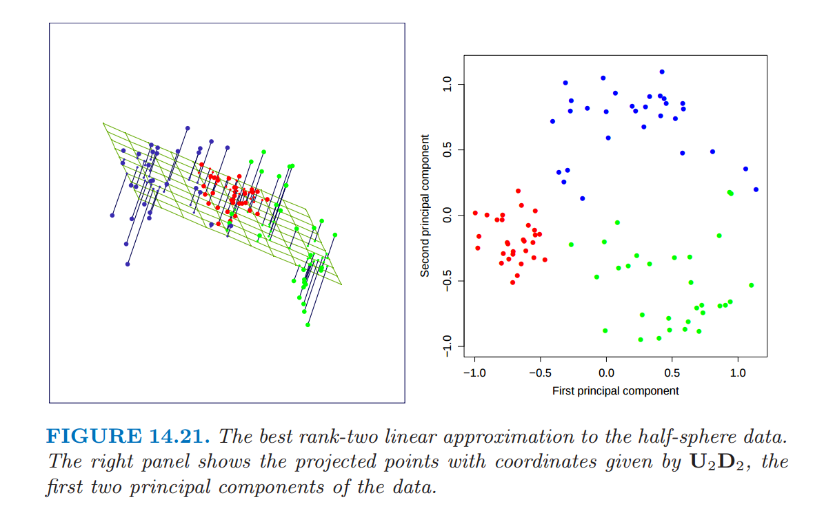
Dimensionality reduction with PCA
\[T_k = U_k D_k\]
where \(U_k\) is a matrix with \(k\) first columns of \(U\) and \(D_k\) is the diagonal matrix containing first \(q\) diagonal terms of \(D\)
The US crime rates dataset
The built in dataset includes information on violent crime rates in the US in 1975.
##            Murder Assault UrbanPop Rape
## Alabama      13.2     236       58 21.2
## Alaska       10.0     263       48 44.5
## Arizona       8.1     294       80 31.0
## Arkansas      8.8     190       50 19.5
## California    9.0     276       91 40.6
## Colorado      7.9     204       78 38.7
Mean and standard deviation of the crime rates across all states:
apply(USArrests, 2, mean)
##   Murder  Assault UrbanPop     Rape
##    7.788  170.760   65.540   21.232
##    Murder   Assault  UrbanPop      Rape
##  4.355510 83.337661 14.474763  9.366385
PCA in R
- In R, the function
prcomp() can be used to perform PCA.
prcomp() is faster and preferred method over princomp(); it is a PCA implementation based on SVD.
pca.res <- prcomp(USArrests, scale = TRUE)
- The output of
prcomp() is a list containing:
## [1] "sdev" "rotation" "center" "scale" "x"
The elements of prcomp output are:
- The principal components/scores matrix, \(T = U\Sigma\) with projected samples coordinates.
##                   PC1        PC2         PC3          PC4
## Alabama    -0.9756604  1.1220012 -0.43980366  0.154696581
## Alaska     -1.9305379  1.0624269  2.01950027 -0.434175454
## Arizona    -1.7454429 -0.7384595  0.05423025 -0.826264240
## Arkansas    0.1399989  1.1085423  0.11342217 -0.180973554
## California -2.4986128 -1.5274267  0.59254100 -0.338559240
## Colorado   -1.4993407 -0.9776297  1.08400162  0.001450164
These are the sample coordinates in the PCA projection space.
- The principal axes matrix, \(V\), contains the eigenvectors of the covariance matrix. A related matrix of loadings is a matrix of eigenvectors scaled by the square roots of the respective eigenvalues:
\[L = \frac{V \Sigma}{\sqrt{n-1}}\]
The loadings or principal axes give the weights of the variables in each of the principal components.
##                 PC1        PC2        PC3         PC4
## Murder   -0.5358995  0.4181809 -0.3412327  0.64922780
## Assault  -0.5831836  0.1879856 -0.2681484 -0.74340748
## UrbanPop -0.2781909 -0.8728062 -0.3780158  0.13387773
## Rape     -0.5434321 -0.1673186  0.8177779  0.08902432
##                 PC1        PC2        PC3         PC4
## Murder   -0.5358995  0.4181809 -0.3412327  0.64922780
## Assault  -0.5831836  0.1879856 -0.2681484 -0.74340748
## UrbanPop -0.2781909 -0.8728062 -0.3780158  0.13387773
## Rape     -0.5434321 -0.1673186  0.8177779  0.08902432
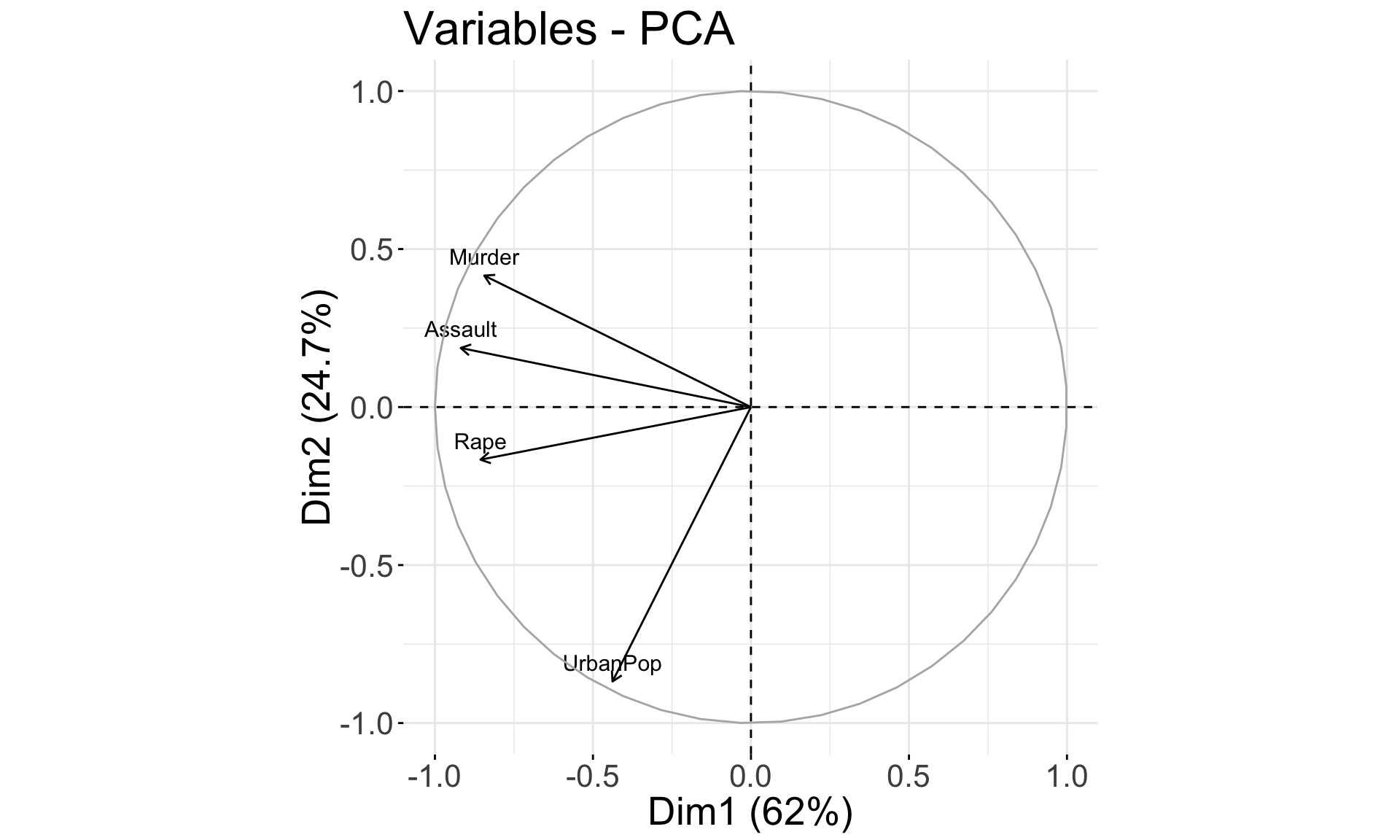
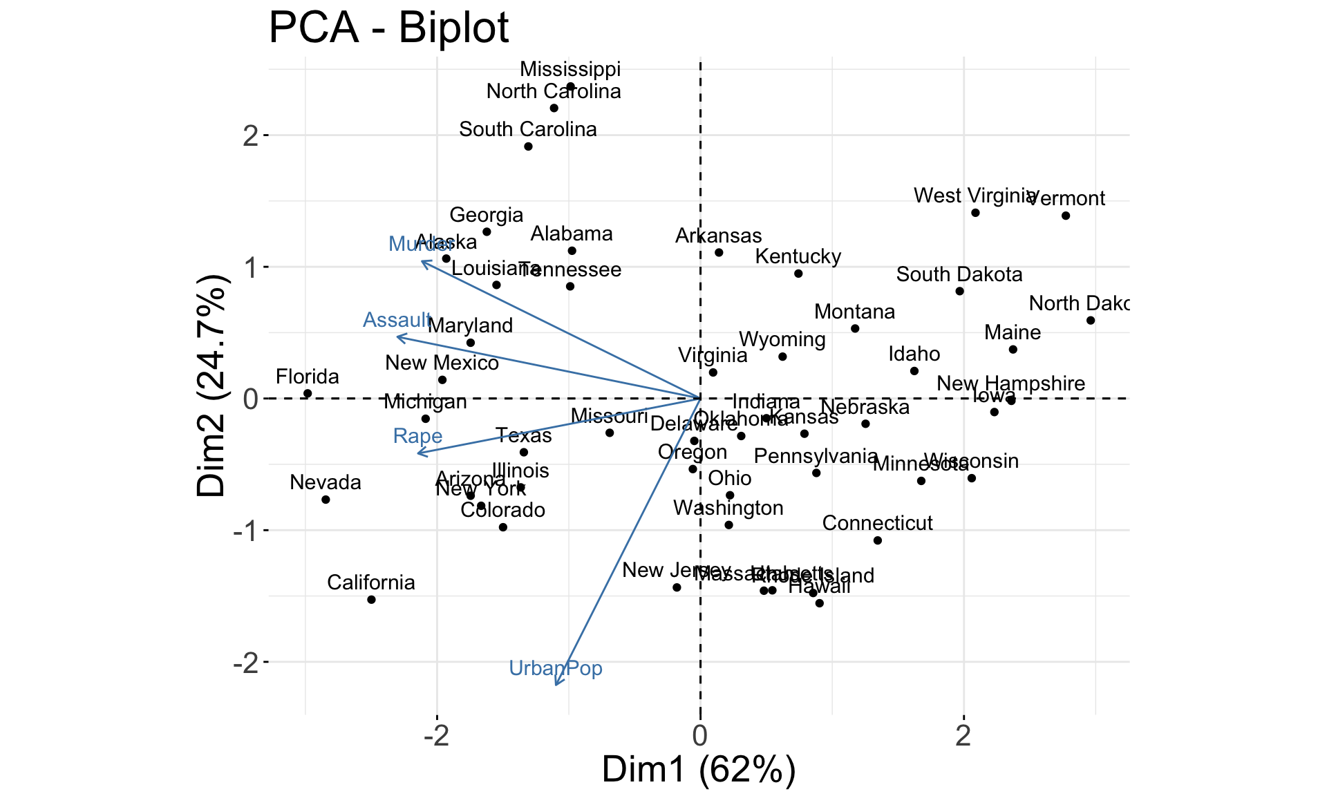
- PC1 places similar weights on
Assault, Murder, and Rape variables, and a much smaller one on UrbanPop. Therefore, PC1 measures an overall measure of crime.
- The 2nd loading puts most weight on
UrbanPop. Thus, PC2 measures a level of urbanization.
- The crime-related variables are correlated with each other, and therefore are close to each other on the biplot.
UrbanPop is independent of the crime rate, and so it is further away on the plot.
- The standard deviations of the principal components (square roots of the eigenvalues of \(\tilde X^T \tilde X\))
## [1] 1.5748783 0.9948694 0.5971291 0.4164494
- The centers of the features, used for shifting:
##   Murder  Assault UrbanPop     Rape
##    7.788  170.760   65.540   21.232
- The standard deviations of the features, used for scaling:
##    Murder   Assault  UrbanPop      Rape
##  4.355510 83.337661 14.474763  9.366385
Scree plot
A scree plot can be used to choose how many components to retain.
Look for “elbows” in the scree plots
Discard the dimensions with corresponding eigenvalues or equivalently the proportion of variance explained that drop off significantly.
# PCA eigenvalues/variances:
(pr.var <- pca.res$sdev^2)
## [1] 2.4802416 0.9897652 0.3565632 0.1734301
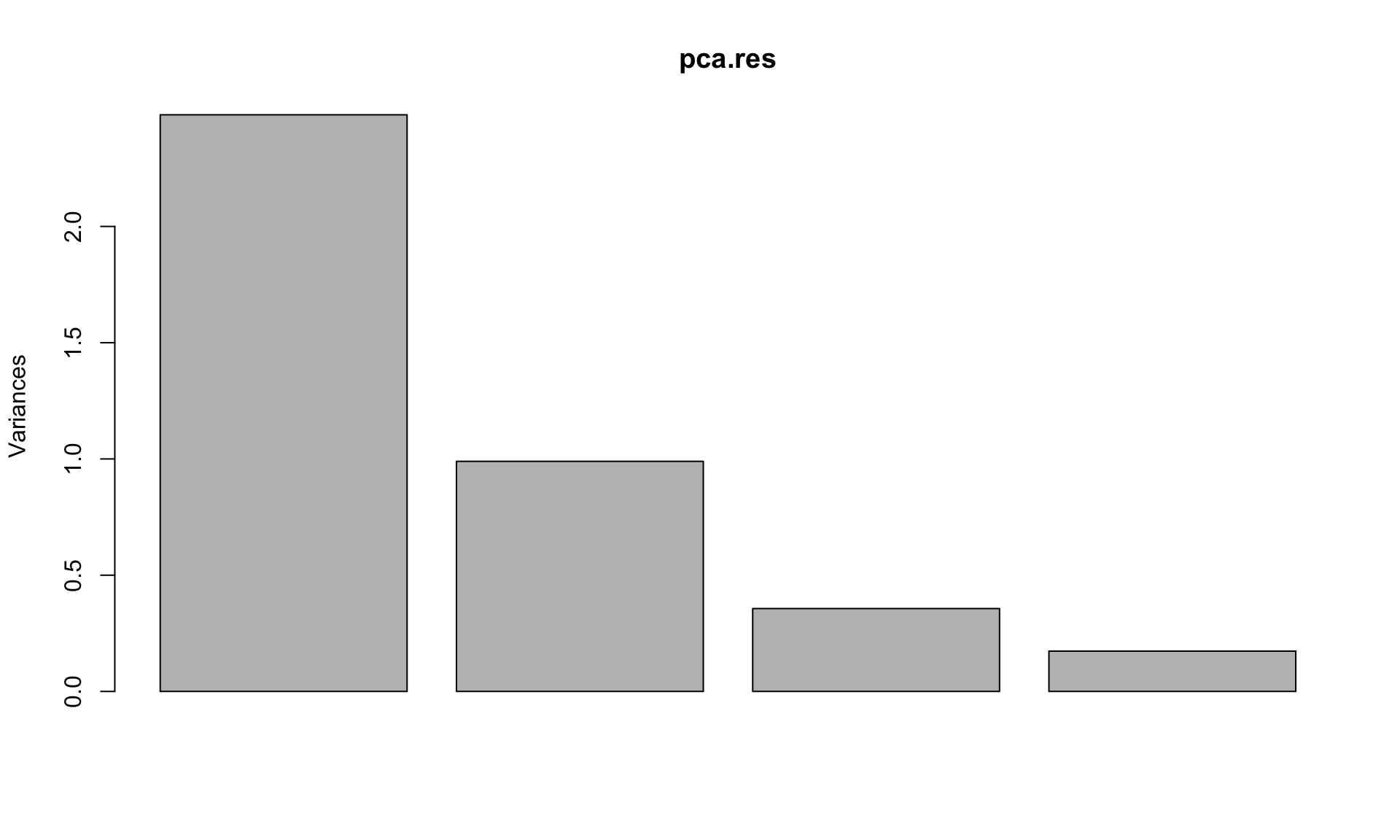
- Percent of variance explained:
# install.packages("factoextra")
library(factoextra)

# Percent of variance explained:
(pve <- 100*pr.var/sum(pr.var))
## [1] 62.006039 24.744129 8.914080 4.335752
fviz_eig(pca.res) + theme(text = element_text(size = 20))

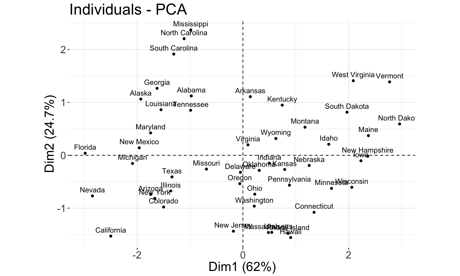
Samples Plot
Each principal component loading and score vector is unique, up to a sign flip. So another software could return this plot instead:
fviz_pca_ind(pca.res) + coord_fixed() +
    theme(text = element_text(size = 20))
Features Plot
fviz_pca_var(pca.res) + coord_fixed() +
    theme(text = element_text(size = 20))
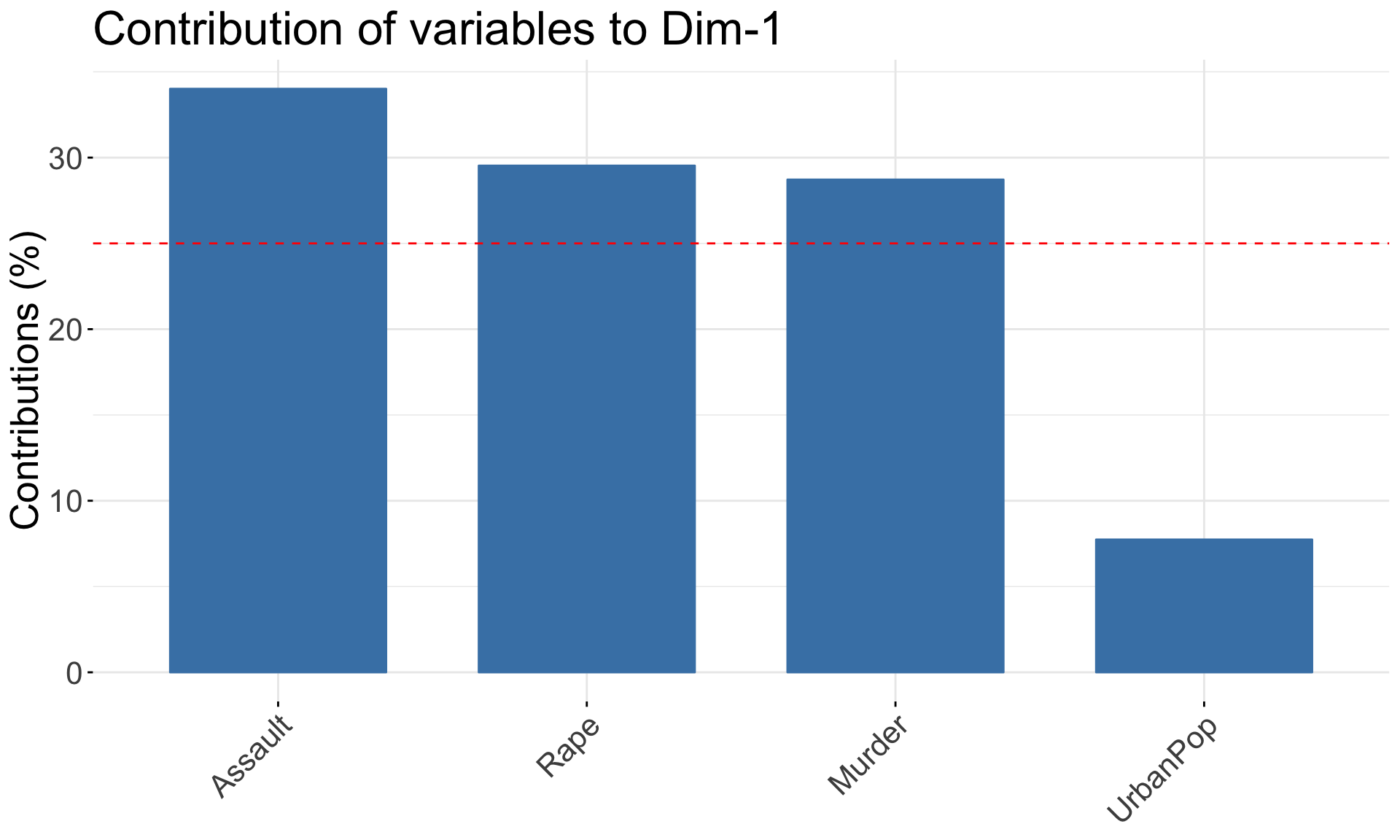
fviz_contrib(pca.res, choice = "var", axes = 1) +
    theme(text = element_text(size = 20))
Biplot
A biplot allows information on both samples and variables of a data matrix to be displayed at the same time.
fviz_pca_biplot(pca.res) + coord_fixed() +
    theme(text = element_text(size = 20))
Cluster Analysis
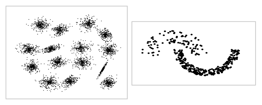
Clustering is an exploratory technique which can discover hidden groups that are important for understanding the data.
Groupings are determined from the data itself, without any prior knowledge about labels or classes.
There are the clustering methods available; a lot of them have an R implementation available on CRAN.
- To cluster the data we need a measure of similarity or dissimilarity between a pair of observations, e.g. an Euclidean distance.
k-means
- k-means is a simple and fast iterative relocation method for clustering data into \(k\) distinct non-overlapping groups.
- The algorithm minimizes the variation within each cluster.
k-means drawbacks
The number clusters \(k\) must be prespecified (before clustering).
The method is stochastic, and involves random initialization of cluster centers.
This means that each time the algorithm is run, the results obtained can be different.
The number of clusters, \(k\), should be chosen using statistics such as:
Importing image to R
- First, we download the image:
library(jpeg)
url <- "http://www.infohostels.com/immagini/news/2179.jpg"
dFile <- download.file(url, "./Lecture8-figure/Image.jpg")
img <- readJPEG("./Lecture8-figure/Image.jpg")
(imgDm <- dim(img))
## [1] 480 960 3
The image is a 3D array, so we will convert it to a data frame.
Each row of the data frame should correspond a single pixel.
The columns should include the pixel location (x and y), and the pixel intensity in red, green, and blue ( R, G, B).
# Assign RGB channels to data frame
imgRGB <- data.frame(
  x = rep(1:imgDm[2], each = imgDm[1]),
  y = rep(imgDm[1]:1, imgDm[2]),
  R = as.vector(img[,,1]),
  G = as.vector(img[,,2]),
  B = as.vector(img[,,3])
)
k-means in R
- Each pixel is a datapoint in 3D specifying the intensity in each of the three “R”, “G”, “B” channels, which determines the pixel’s color.
##   x   y R         G         B
## 1 1 480 0 0.3686275 0.6980392
## 2 1 479 0 0.3686275 0.6980392
## 3 1 478 0 0.3725490 0.7019608
- We use k-means to cluster the pixels \(k\) into color groups (clusters).
- k-means can be performed in R with
kmeans() built-in function.
# Set seed since k-means involves a random initialization
set.seed(43658)
k <- 2
kmeans.2clust <- kmeans(imgRGB[, c("R", "G", "B")], centers = k)
names(kmeans.2clust)
## [1] "cluster"      "centers"      "totss"        "withinss"
## [5] "tot.withinss" "betweenss"    "size"         "iter"
## [9] "ifault"
# k cluster centers
kmeans.2clust$centers
##           R         G         B
## 1 0.5682233 0.3251528 0.1452832
## 2 0.6597320 0.6828609 0.7591578
# The centers correspond to the following colors:
rgb(kmeans.2clust$centers)
## [1] "#915325" "#A8AEC2"
# Cluster assignment of the first 10 pixels
head(kmeans.2clust$cluster, 10)
## [1] 2 2 2 2 2 2 2 2 2 2
# Convert cluster assignment lables to cluster colors
kmeans.2colors <- rgb(kmeans.2clust$centers[kmeans.2clust$cluster, ])
head(kmeans.2colors, 10)
##  [1] "#A8AEC2" "#A8AEC2" "#A8AEC2" "#A8AEC2" "#A8AEC2" "#A8AEC2" "#A8AEC2"
##  [8] "#A8AEC2" "#A8AEC2" "#A8AEC2"
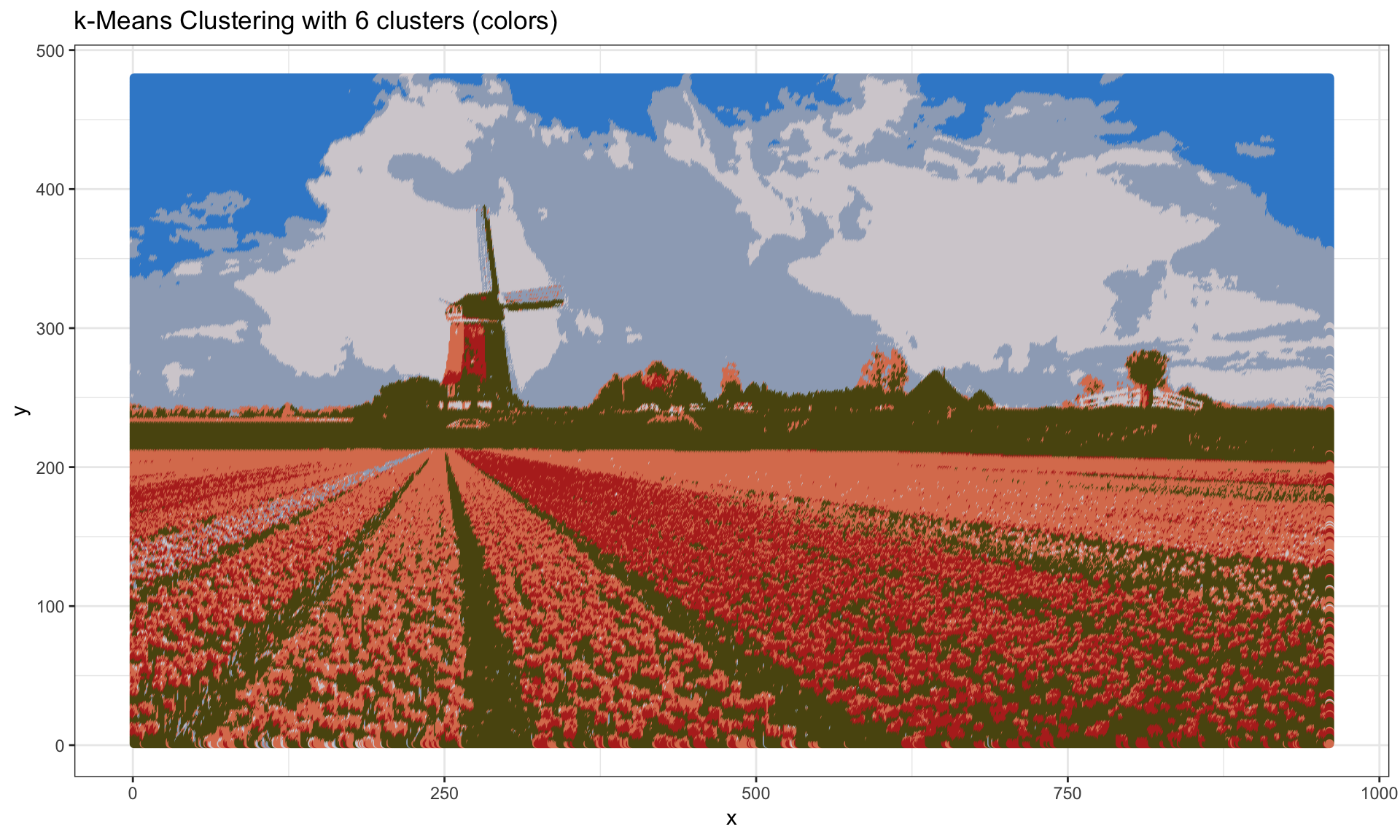
ggplot(data = imgRGB, aes(x = x, y = y)) +
  geom_point(colour = kmeans.2colors) +
  labs(title = paste("k-Means Clustering with", k, "clusters (colors)")) +
  xlab("x") + ylab("y") + theme_bw()

Now add more colors, by increase the number of clusters to 6:
set.seed(348675)
kmeans.6clust <- kmeans(imgRGB[, c("R", "G", "B")], centers = 6)
kmeans.6colors <- rgb(kmeans.6clust$centers[kmeans.6clust$cluster, ])
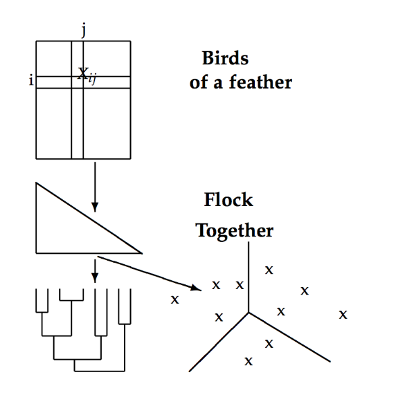
Hierarchical clustering
Alexander Calder’s mobile
- If it’s difficult (or if you simply don’t want) to choose the number of clusters ahead, you can do hierarchical clustering.
Hierarchical clustering can be performed using agglomerative (bottom-up) or divisive (top-down) approach.
The method requires a choice of a pairwise distance metric and a rule of how to merge or divide clusters.
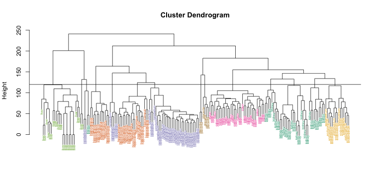
The output of the method can be represented as a graphical tree-based representation of the data, called a dendogram.
The tree allows you to evaluate where the cutoff for grouping should occur.
Hierarchical clustering algorithm
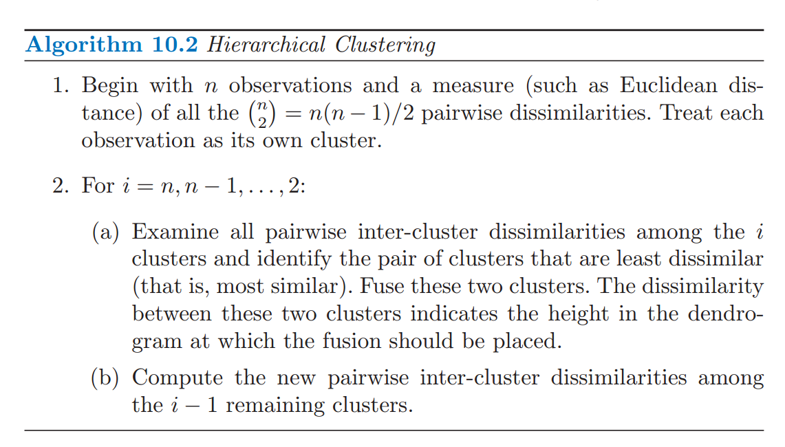
Source: ISL
Results for hierarchical clustering differ depending on the choice of:
A distance metric used for pairs of observations, e.g. Euclidean (L2), Manhattan (L1), Jaccard (Binary), etc
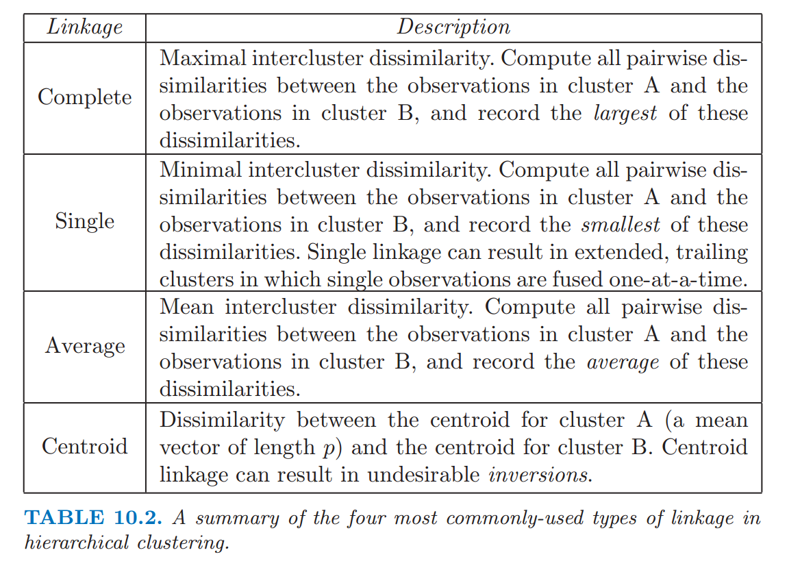
The rule used for grouping clusters that are already generated, e.g. single (minimum), completer (maximum), centroid or average cluster linkages.
Different ways to compute dissimilarity between 2 clusters:
Iris dataset
- We will use the Fisher’s Iris dataset containing measurements on 150 irises.
- Hierarchical clustering will calculate the grouping of the flowers into groups corresponding. We will see that these groups will roughly correspond to the flower species.
##   Sepal.Length Sepal.Width Petal.Length Petal.Width Species
## 1          5.1         3.5          1.4         0.2  setosa
## 2          4.9         3.0          1.4         0.2  setosa
## 3          4.7         3.2          1.3         0.2  setosa
## 4          4.6         3.1          1.5         0.2  setosa
## 5          5.0         3.6          1.4         0.2  setosa
## 6          5.4         3.9          1.7         0.4  setosa
Hierarchical clustering in R
- Built-in function
hclust() performs hierarchical clustering.
- We will use only the petal dimensions (2 columns) to compute the distances between flowers.
# We use the Euclidean distance for the dissimilarities between flowers
distMat <- dist(iris[, 3:4])


# We use the "complete" linkage method for computing the cluster distances.
clusters <- hclust(distMat, method = "complete")
plot(clusters, cex = 0.7)
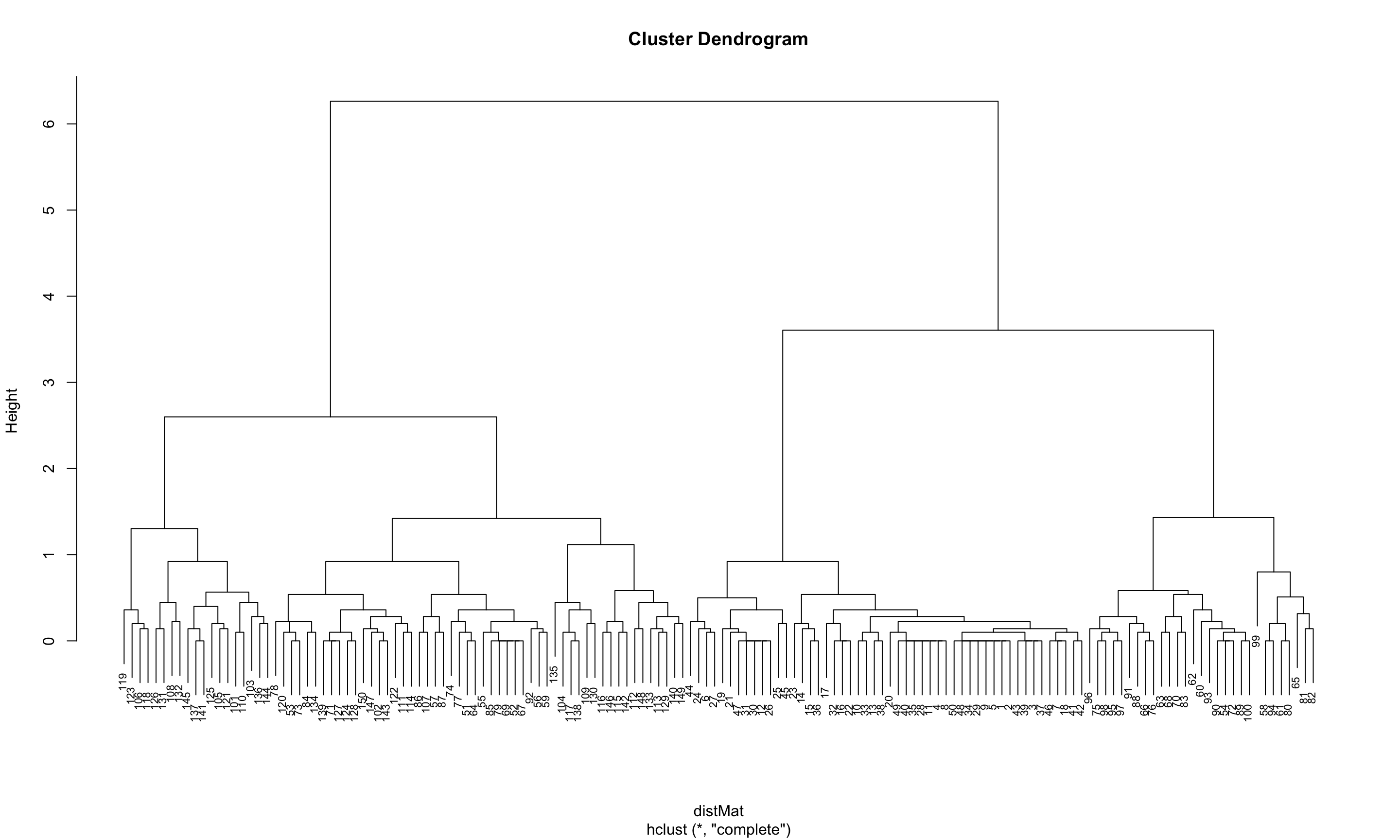
The dendrogram suggests that a reasonable choice of the number of clusters is either 3 or 4.
plot(clusters, cex = 0.7)
abline(a = 2, b = 0, col = "blue")
abline(a = 3, b = 0, col = "blue")

- We pick 3 clusters.
- To get the assignments with 3 clusters from the truncated tree we can use a
cutree() function.
(clusterCut <- cutree(clusters, 3))
##   [1] 1 1 1 1 1 1 1 1 1 1 1 1 1 1 1 1 1 1 1 1 1 1 1 1 1 1 1 1 1 1 1 1 1 1 1
##  [36] 1 1 1 1 1 1 1 1 1 1 1 1 1 1 1 2 2 2 3 2 2 2 3 2 3 3 3 3 2 3 3 2 3 2 3
##  [71] 2 3 2 2 3 3 2 2 2 3 3 3 3 2 2 2 2 3 3 3 3 2 3 3 3 3 3 3 3 3 2 2 2 2 2
## [106] 2 2 2 2 2 2 2 2 2 2 2 2 2 2 2 2 2 2 2 2 2 2 2 2 2 2 2 2 2 2 2 2 2 2 2
## [141] 2 2 2 2 2 2 2 2 2 2
table(clusterCut, iris$Species)
##
## clusterCut setosa versicolor virginica
##          1     50          0         0
##          2      0         21        50
##          3      0         29         0
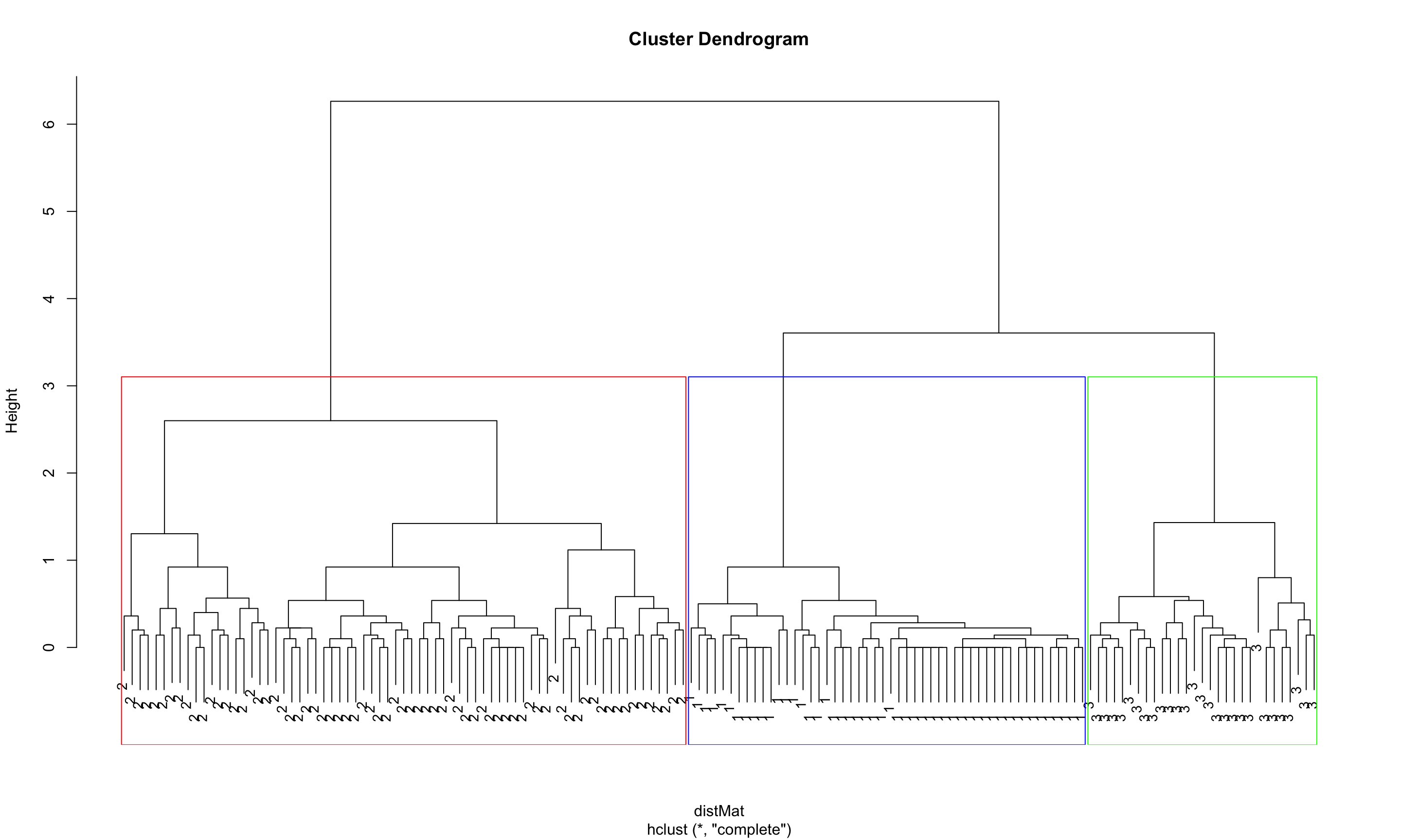
plot(clusters, labels = clusterCut, cex = 0.9)
rect.hclust(clusters, k = 3, border=c("red", "blue", "green"))
table(clusterCut, iris$Species)
##
## clusterCut setosa versicolor virginica
##          1     50          0         0
##          2      0         21        50
##          3      0         29         0
- From the table we see that the sentosa and virginica were correctly assigned to separate groups.
- However, the method had difficulty grouping the versicolorm flowers into a separate cluster.
Try another linkage method like “average” and see if it performs better.
# We use the Euclidean distance for the dissimilarities between flowers
distMat <- dist(iris[, 3:4])
# We use the "complete" linkage method for computing the cluster distances.
clusters <- hclust(distMat, method = "average")
plot(clusters, cex = 0.5)
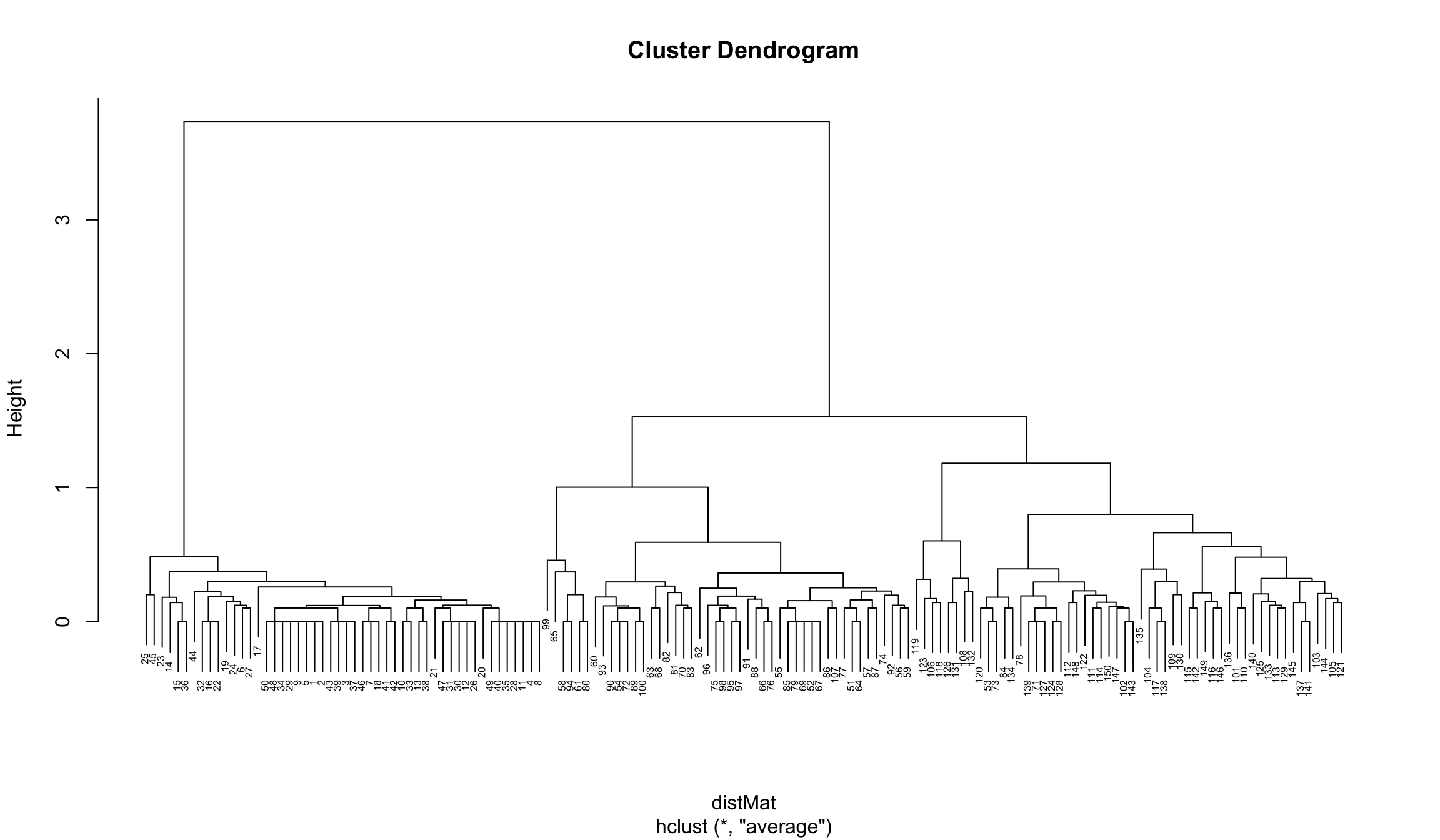
Here we can choose 3 or 5 clusters:
plot(clusters, cex = 0.6)
abline(a = 1.35, b = 0, col = "blue")
abline(a = 0.9, b = 0, col = "blue")
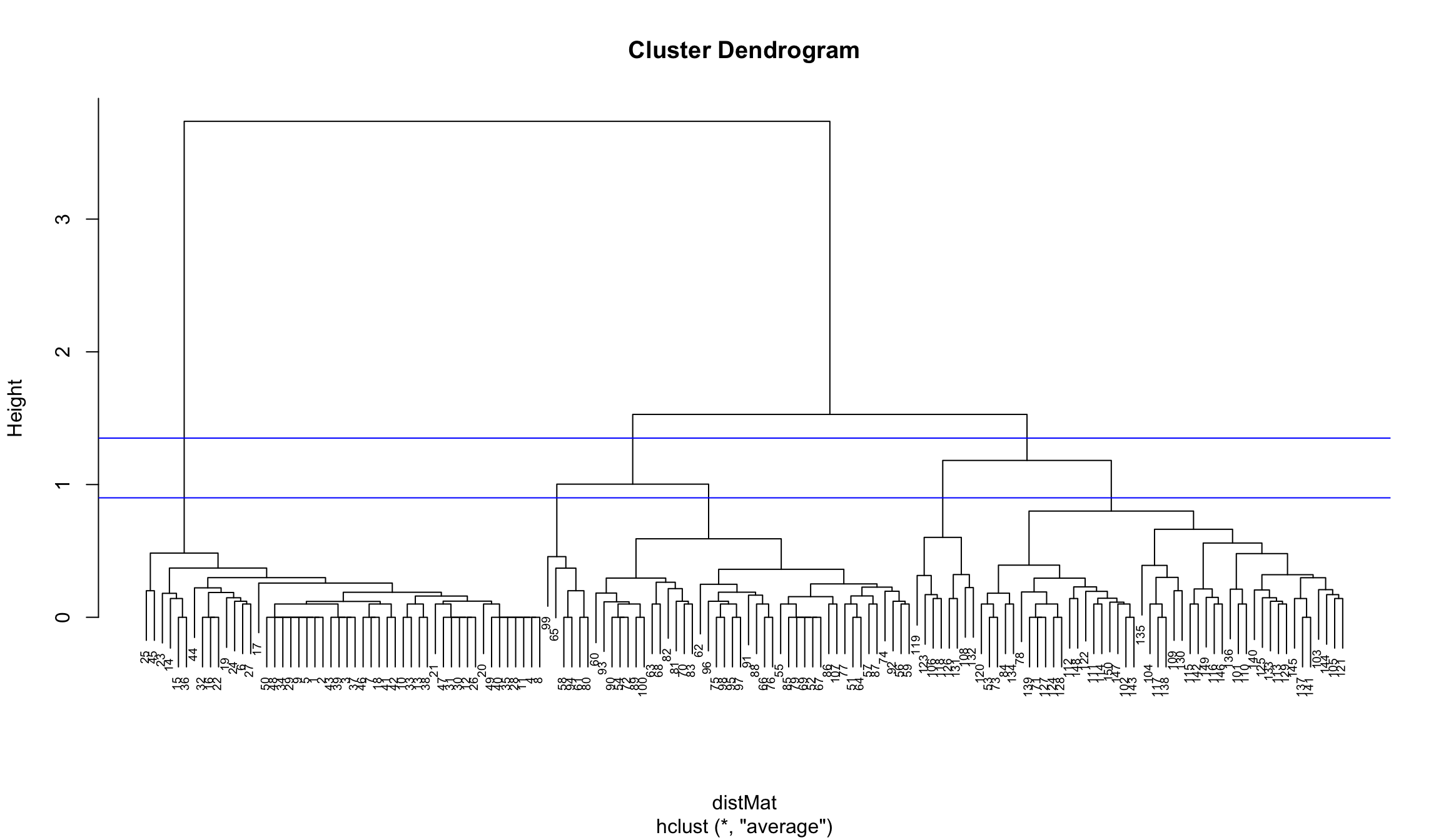
Again we choose 3 clusters
clusterCut <- cutree(clusters, 3)
table(clusterCut, iris$Species)
##
## clusterCut setosa versicolor virginica
##          1     50          0         0
##          2      0         45         1
##          3      0          5        49
We see that this time the results are better in terms of the cluster assignment agreement with the flower species classification.
plot(clusters, labels = clusterCut, cex = 0.7)
rect.hclust(clusters, k = 3, border=c("red", "blue", "green"))

- 2D plot of the iris dataset using petal dimensions as coordinates.
- The cluster assignments partition the flowers into species with high accuracy.
ggplot(iris, aes(Petal.Length, Petal.Width)) + theme_bw() +
  geom_text(aes(label = clusterCut), vjust = -1) +
  geom_point(aes(color = Species)) + coord_fixed(1.5)

Multidimensional Scaling
MDS algorithm aims to place each object in N-dimensional space such that the between-object distances are preserved as well as possible. Each object is then assigned coordinates in each of the N dimensions. The number of dimensions of an MDS plot N can exceed 2 and is specified a priori. Choosing N=2 optimizes the object locations for a two-dimensional scatterplot.
There are different types of MDS methods including, Classical MDS, Metric MDS and Non-metric MDS. The details on the differences ca be found on:
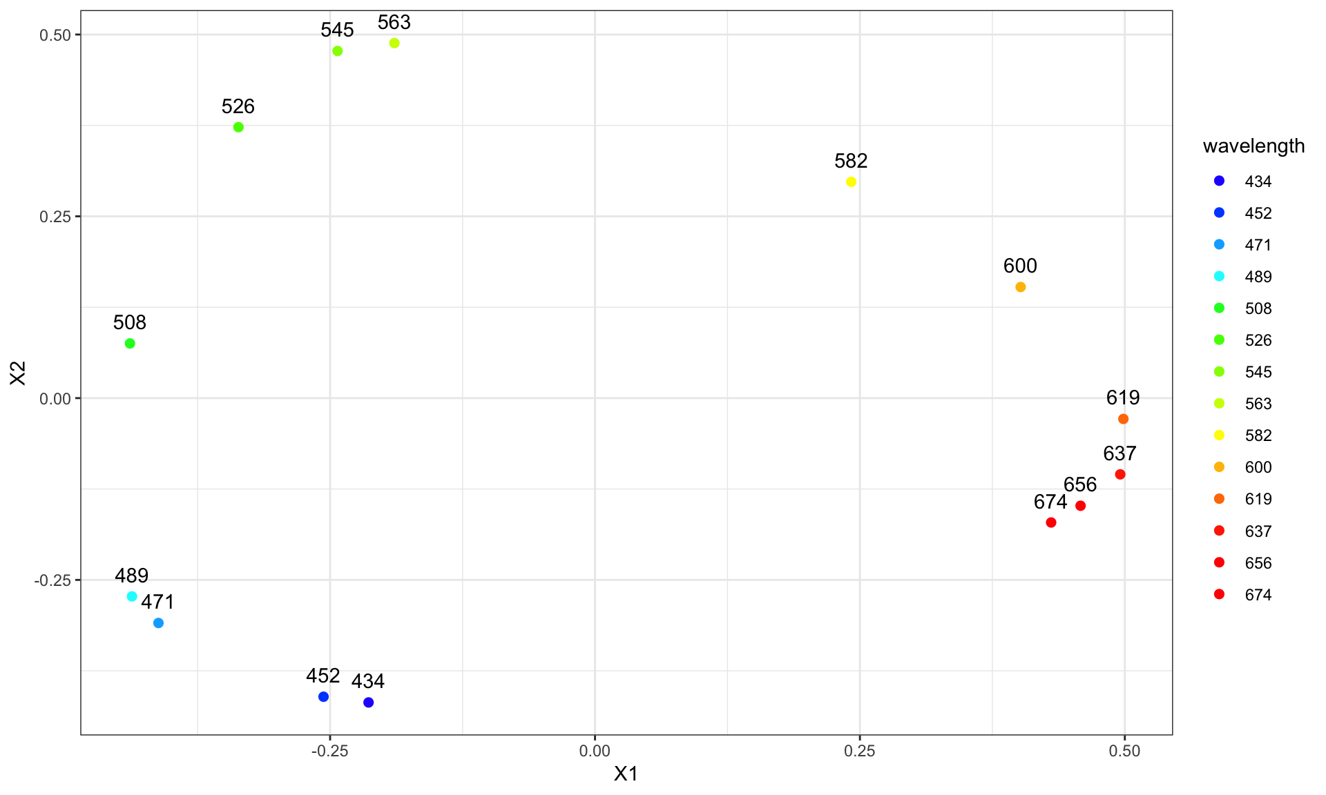
Perception of colors
- Gosta Ekman studied how people perceive colors in his paper from 1954.
- He collected survey data from 31 subjects, which included participants’ rating of the dissimilarity between each pair of 14 colors on a 5-point scale.
- The ratings of all subjects were averaged, and the final mean dissimilarity matrix was used for constructing “map of colors”.
14 colors were studied with wavelengths in the range between 434 and 674 nm.
# color similarity scores
ekmanSim <- readRDS("./Lecture8-figure/ekman.rds")
print(ekmanSim)
##      434  445  465  472  490  504  537  555  584  600  610  628  651
## 445 0.86
## 465 0.42 0.50
## 472 0.42 0.44 0.81
## 490 0.18 0.22 0.47 0.54
## 504 0.06 0.09 0.17 0.25 0.61
## 537 0.07 0.07 0.10 0.10 0.31 0.62
## 555 0.04 0.07 0.08 0.09 0.26 0.45 0.73
## 584 0.02 0.02 0.02 0.02 0.07 0.14 0.22 0.33
## 600 0.07 0.04 0.01 0.01 0.02 0.08 0.14 0.19 0.58
## 610 0.09 0.07 0.02 0.00 0.02 0.02 0.05 0.04 0.37 0.74
## 628 0.12 0.11 0.01 0.01 0.01 0.02 0.02 0.03 0.27 0.50 0.76
## 651 0.13 0.13 0.05 0.02 0.02 0.02 0.02 0.02 0.20 0.41 0.62 0.85
## 674 0.16 0.14 0.03 0.04 0.00 0.01 0.00 0.02 0.23 0.28 0.55 0.68 0.76
# convert similarities to dissimilarities
ekmanDist <- 1 - ekmanSim
MDS in R
- Use
cmdscale() built-in function for classical MDS.
- Metric iterative MDS and non-metric MDS function are available in a package
smacof and other packages are also compared here.
ekmanMDS <- cmdscale(ekmanDist, k = 2)
res <- data.frame(ekmanMDS)
head(res)
##             X1          X2
## 434 -0.2137161 -0.41852576
## 445 -0.2562012 -0.41065436
## 465 -0.4119890 -0.30925977
## 472 -0.4369586 -0.27266935
## 490 -0.4388604  0.07518594
## 504 -0.3364868  0.37262279
library("ggplot2")
wavelengths <- round(seq( 434, 674, length.out = 14))
res$wavelength <- factor(wavelengths, levels =wavelengths)
ggplot(res, aes(X1, X2)) + geom_point() + theme_bw() +
  geom_text(aes(label = wavelength), vjust=-1)

The wavelengths were converted to hexadecimal colors using this website.
hex <- c("#2800ff", "#0051ff", "#00aeff", "#00fbff", "#00ff28", "#4eff00", "#92ff00",
          "#ccff00", "#fff900", "#ffbe00", "#ff7b00", "#ff3000", "#ff0000", "#ff0000")
ggplot(res, aes(X1, X2)) + theme_bw() +
  geom_point(aes(color = wavelength), size = 2) +
  geom_text(aes(label = wavelength), vjust=-1) +
  scale_color_manual(values = hex)
t-Distributed Stochastic Neighbor Embedding
- t-SNE is a nonlinear technique developed by van der Maaten and Hinton for dimensionality reduction
- It is particularly well suited for the visualization of high-dimensional datasets.
- The method performs well at visualizing and exposing inherent data clusters
- It has been widely applied in many fields including genomics, where the method is commonly used in single-cell literature for visualizing cell subpopulations.
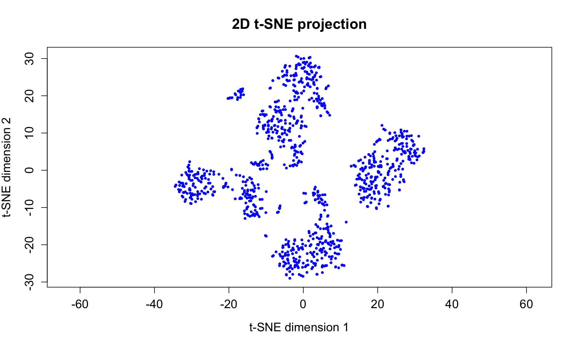
tSNE on mass cytometry data
The following example shows how to calculate and plot a 2D t-SNE projection using the Rtsne package. The example and code was developed by Lukas Weber.
- The dataset used is the mass cytometry of healthy human bone marrow dataset from the study conducted by Amir et al. (2013).
- Mass cytometry measures the expression levels of up to 40 proteins per cell and hundreds of cells per second.
- In this example t-SNE is very effective at displaying groups of different cell populations (types).
#  here we use a subset of the data
path <- "./Lecture8-figure/healthyHumanBoneMarrow_small.csv"
dat <- read.csv(path)
# We select 13 protein markers to used in Amir et al. 2013
colnames_proj <- colnames(dat)[c(11, 23, 10, 16, 7, 22, 14, 28, 12, 6, 8, 13, 30)]
dat <- dat[, colnames_proj]
head(dat)
##   X144.CD11b X160.CD123  X142.CD19  X147.CD20 X110.111.112.114.CD3
## 1   5.967343 14.0255518  0.5294468  5.0397625           149.204117
## 2  -2.965949 -0.4499034 -0.9504946  3.2883098           102.398453
## 3  22.475813  7.9440827 -2.5556924 -0.3310032            -9.759324
## 4  -5.457655 -0.3668855 -0.8048915  1.7649024           146.526154
## 5 127.534332 13.2033119  0.7140800 -1.0700325             7.266849
## 6  12.181891  9.0580482  1.9163597  2.1253521           653.283997
##     X158.CD33  X148.CD34  X167.CD38    X145.CD4 X115.CD45 X139.CD45RA
## 1   2.4958646  4.3011222  29.566343   0.8041515 606.56268  291.058655
## 2   0.3570583  1.3665982  26.355003  -0.2354967 192.41901   -1.998943
## 3 304.6151733  3.0677378 165.949097   0.3407812  98.22443    5.670944
## 4  -2.2423408 -0.7205721   3.933757  -0.6418993 482.09525   13.697150
## 5 343.4721985 -0.9823112 193.646225  30.6597385 212.06926    6.608723
## 6   3.9792464 -1.5659959 163.225845 152.5955353 284.07599   36.927834
##      X146.CD8 X170.CD90
## 1 346.5215759 12.444887
## 2  35.8152542 -0.615051
## 3   0.8252113 13.740484
## 4 155.2028503  8.284868
## 5   2.1295056 10.848905
## 6  14.1040640  6.430328
# arcsinh transformation
# (see Amir et al. 2013, Online Methods, "Processing of mass cytometry data")
asinh_scale <- 5
dat <- asinh(dat / asinh_scale)
# prepare data for Rtsne
dat <- dat[!duplicated(dat), ]  # remove rows containing duplicate values within rounding
dim(dat)
## [1] 999 13
library(Rtsne)
# run Rtsne (Barnes-Hut-SNE algorithm) without PCA step
# (see Amir et al. 2013, Online Methods, "viSNE analysis")
set.seed(123)
rtsne_out <- Rtsne(as.matrix(dat), perplexity = 20,
                   pca = FALSE, verbose = FALSE)
# plot 2D t-SNE projection
plot(rtsne_out$Y, asp = 1, pch = 20, col = "blue",
     cex = 0.75, cex.axis = 1.25, cex.lab = 1.25, cex.main = 1.5,
     xlab = "t-SNE dimension 1", ylab = "t-SNE dimension 2",
     main = "2D t-SNE projection")
 Source: link