Lecture 6: Data modeling and linear regression
CME/STATS 195
Lan Huong Nguyen
October 16, 2018
Contents
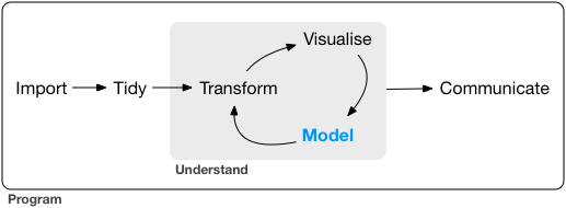
Data Modeling
Linear Regression
Lasso Regression
A toy dataset
We will work with a simulated dataset sim1 from modelr:
sim1## # A tibble: 30 x 2
## x y
## <int> <dbl>
## 1 1 4.20
## 2 1 7.51
## 3 1 2.13
## 4 2 8.99
## 5 2 10.2
## 6 2 11.3
## 7 3 7.36
## 8 3 10.5
## 9 3 10.5
## 10 4 12.4
## # ... with 20 more rowsggplot(sim1, aes(x, y)) + geom_point()
Defining a family of models
The relationship between \(x\) and \(y\) for the points in sim1 look linear. So, will look for models which belong to a family of models of the following form:
\[y= \beta_0 + \beta_1 \cdot x\]
The models that can be expressed by the above formula, can adequately capture a linear trend.
We generate a few examples of the models from this family on the right.
models <- tibble(
    b0 = runif(250, -20, 40),
    b1 = runif(250, -5, 5))

ggplot(sim1, aes(x, y)) +
  geom_abline(
      data = models,
      aes(intercept = b0, slope = b1),
      alpha = 1/4) +
geom_point() 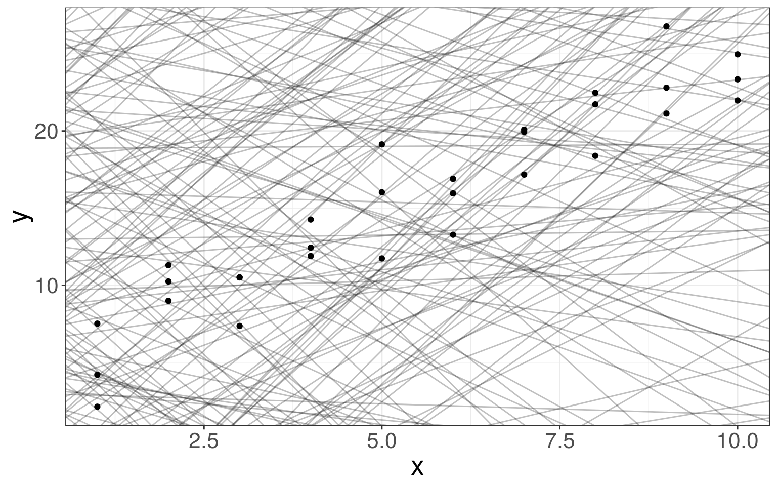
Fitting a model
From all the lines in the linear family of models, we need to find the best one, i.e. the one that is the closest to the data.
This means that we need to find parameters \(\hat a_0\) and \(\hat a_1\) that identify such a fitted line.
The closest to the data can be defined as the one with the minimum distance to the data points in the \(y\) direction (the minimum residuals):
\[\begin{align*} \|\hat e\|^2_2 &= \|\vec y - \hat y\|_2^2\\ &= \|\vec y - (\hat \beta_0 + \hat \beta_1 x)\|_2^2\\ &= \sum_{i = 1}^n (y_i - (\hat \beta_0 + \hat \beta_1 x_i))^2 \end{align*}\]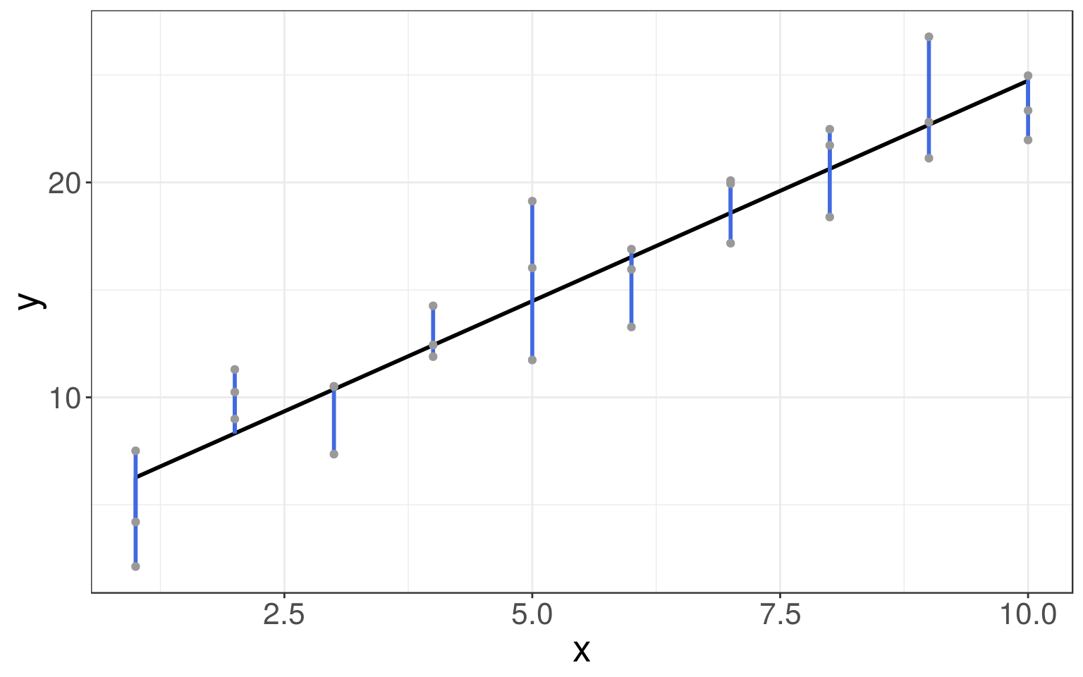
Visualizing the model
Now we can compare our predictions (grey) to the observed (black) values.
ggplot(mtcars_train, aes(wt)) + geom_point(aes(y = mpg)) +
    geom_line(aes(y = pred), color = "red", size = 1) +
geom_point(aes(y = pred), fill = "grey", color = "black", shape = 21, size = 2) 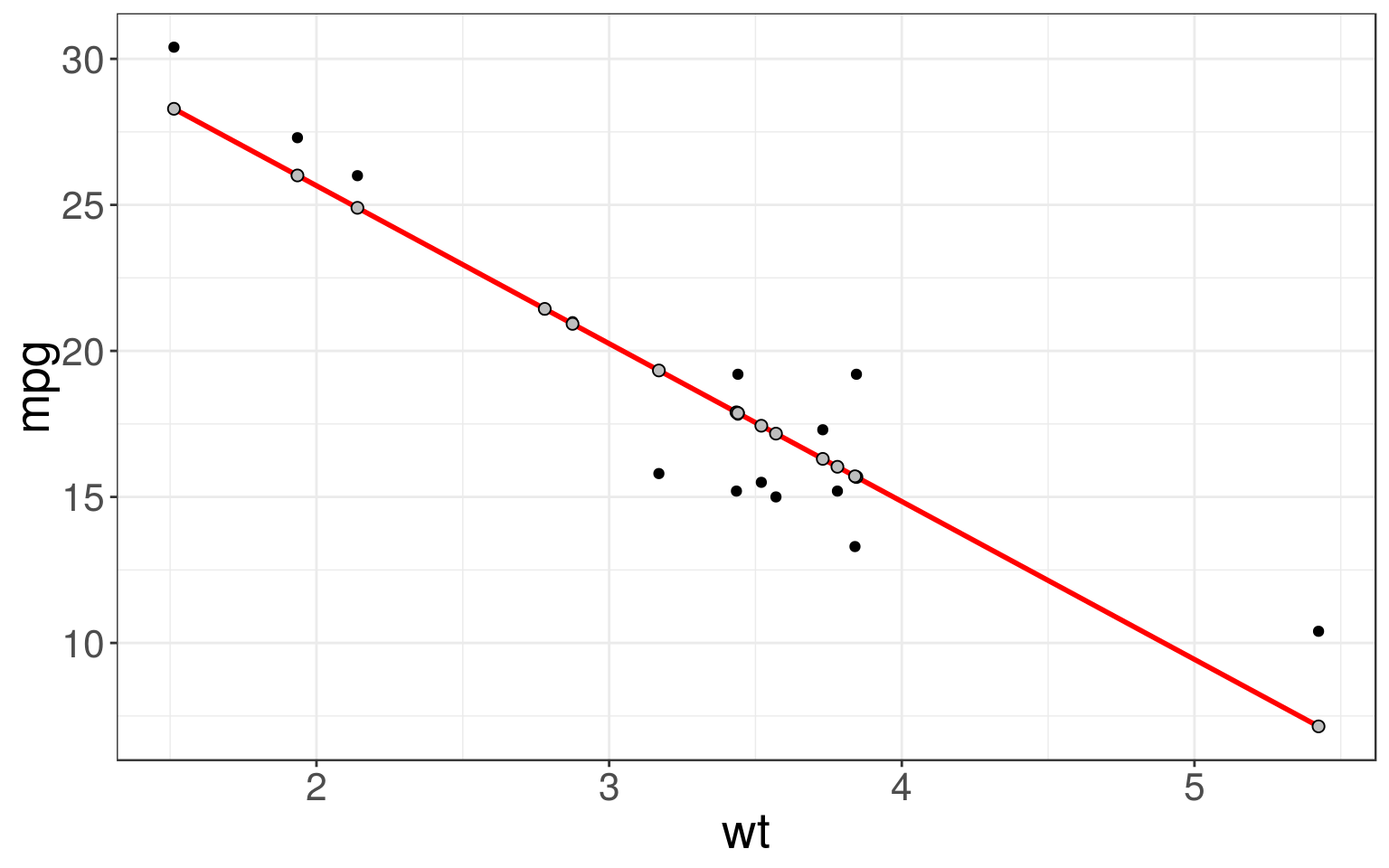
Visualizing the residuals
The residuals tell you what the model has missed. We can compute and add residuals to data with add_residuals() from modelr package:
Plotting residuals is a good practice – you want the residuals to look like random noise.
mtcars_train <- mtcars_train %>%
    add_residuals(mtcars_fit)
mtcars_train %>%
    select(mpg, mpg, resid, pred)
## # A tibble: 16 x 3
## mpg resid pred
## <dbl> <dbl> <dbl>
## 1 19.2 1.33 17.9
## 2 19.2 3.52 15.7
## 3 17.3 0.998 16.3
## 4 27.3 1.29 26.0
## 5 26 1.10 24.9
## 6 21 0.0748 20.9
## 7 15.2 -0.832 16.0
## 8 15.2 -2.70 17.9
## 9 15.8 -3.53 19.3
## 10 17.8 -0.0704 17.9
## 11 15.5 -1.94 17.4
## 12 21.4 -0.0389 21.4
## 13 13.3 -2.41 15.7
## 14 15 -2.17 17.2
## 15 30.4 2.11 28.3
## 16 10.4 3.26 7.14ggplot(mtcars_train, aes(wt, resid)) +
geom_ref_line(h = 0, colour = "grey") +
geom_point() 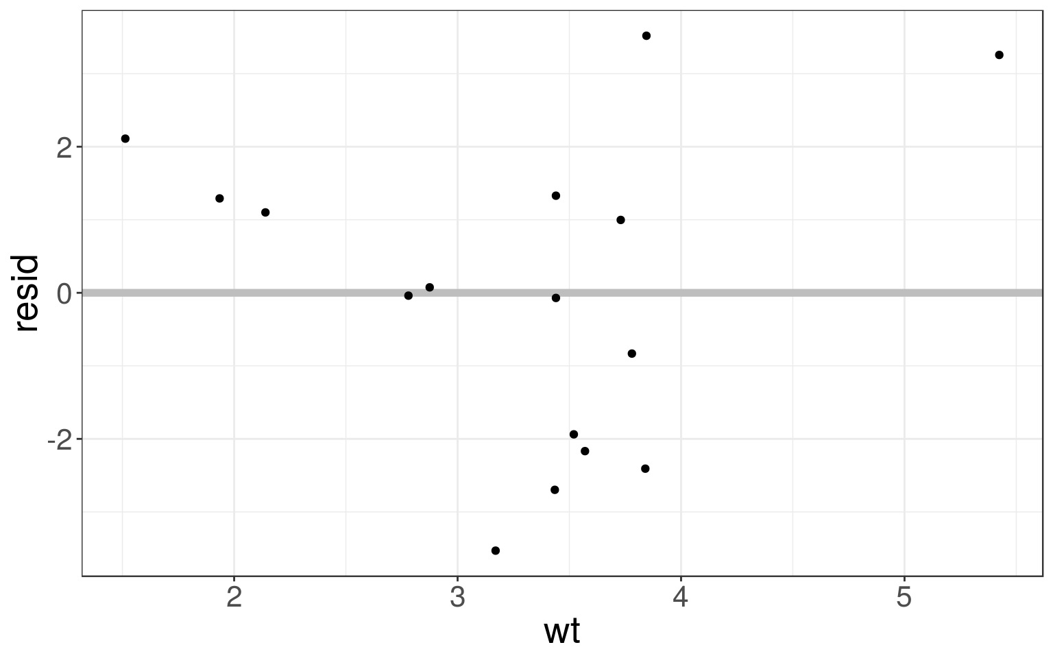
Multiple Linear Regression
Models often include multiple predictors, e.g. we might like to predict mpg using three variables: wt, disp and cyl.
ggplot(mtcars, aes(x=wt, y=mpg, col=cyl, size=disp)) +
    geom_point() +
    scale_color_viridis_c()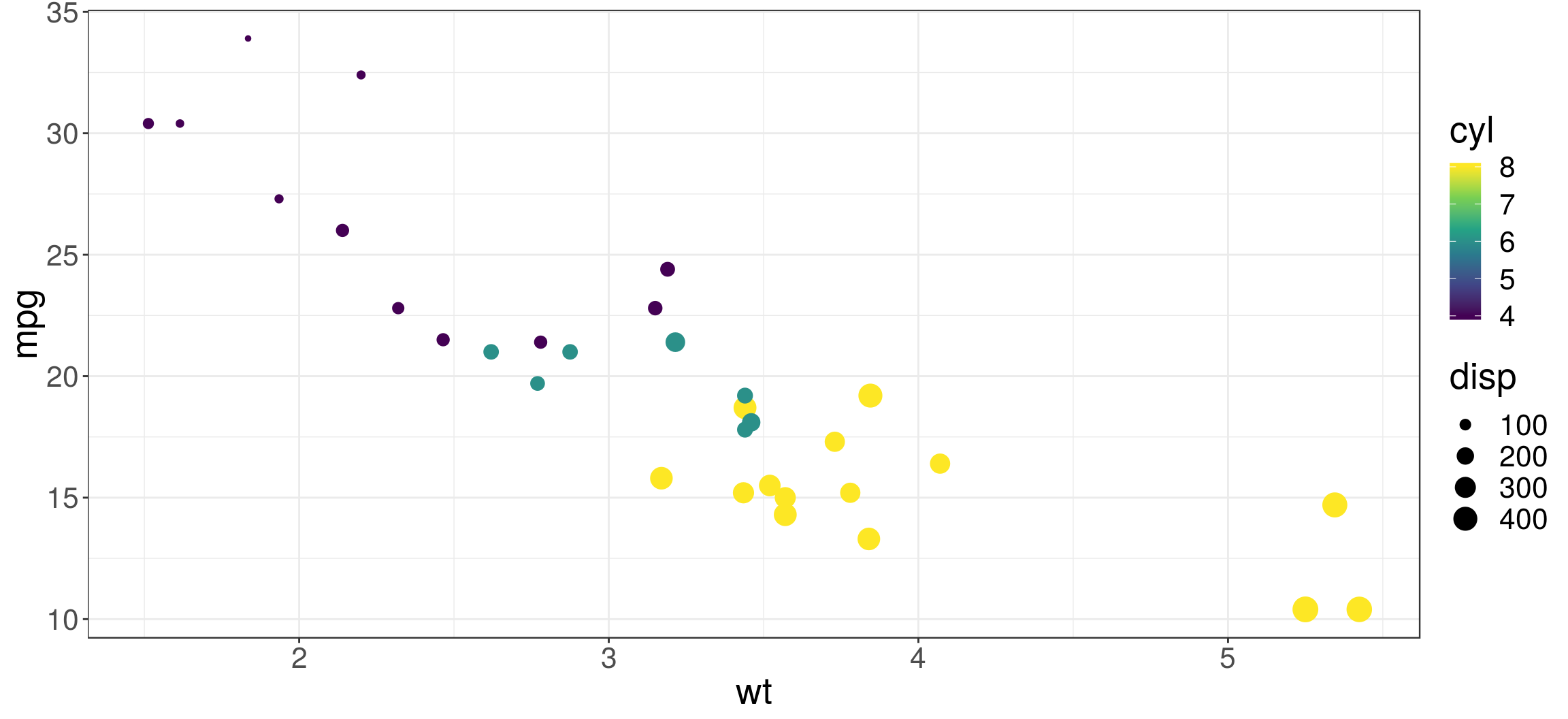
Formulas with interactions
In the sim3 dataset, there is a categorical, x2, and a continuous, x1, predictor.
ggplot(sim3, aes(x=x1, y=y)) + geom_point(aes(color = x2)) 
Models with interactions
We could fit two different models, one without and one with (mod2) different slopes and intercepts for each line (for each x2 category).
# Model without interactions:
mod1 <- lm(y ~ x1 + x2, data = sim3)
# Model with interactions:
mod2 <- lm(y ~ x1 * x2, data = sim3)
# Generate a data grid for two variables
# and compute predictions from both models
grid <- sim3 %>% data_grid(x1, x2) %>%
    gather_predictions(mod1, mod2)
head(grid, 3)
## # A tibble: 3 x 4
## model x1 x2 pred
## <chr> <int> <fct> <dbl>
## 1 mod1 1 a 1.67
## 2 mod1 1 b 4.56
## 3 mod1 1 c 6.48tail(grid, 3)## # A tibble: 3 x 4
## model x1 x2 pred
## <chr> <int> <fct> <dbl>
## 1 mod2 10 b -0.162
## 2 mod2 10 c 5.48
## 3 mod2 10 d 3.98ggplot(sim3, aes(x=x1, y=y, color=x2)) +
geom_point() +
geom_line(data=grid, aes(y=pred)) +
facet_wrap(~ model) 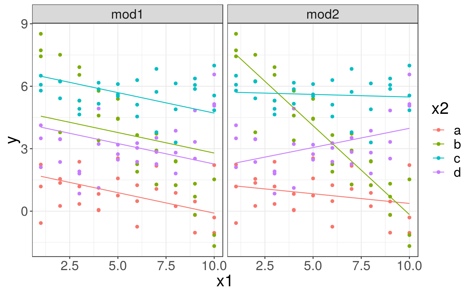
# label = TRUE makes the plot annotate the curves with the corresponding coeffients labels.
plot(fit, label = TRUE, xvar = "lambda") 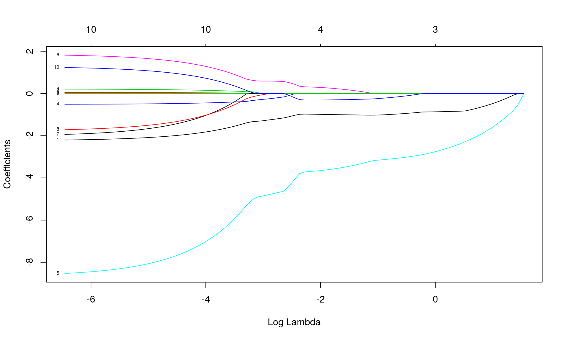
- the y-axis corresponds the value of the coefficients.
- the x-axis is denoted “Log Lambda” corresponds to the value of \(\lambda\) parameter penalizing the L1 norm of \(\boldsymbol{ \hat \beta}\)
set.seed(1)
# `nfolds` argument sets the number of folds (k).
cvfit <- cv.glmnet(X_train, y_train, nfolds = 5)
plot(cvfit)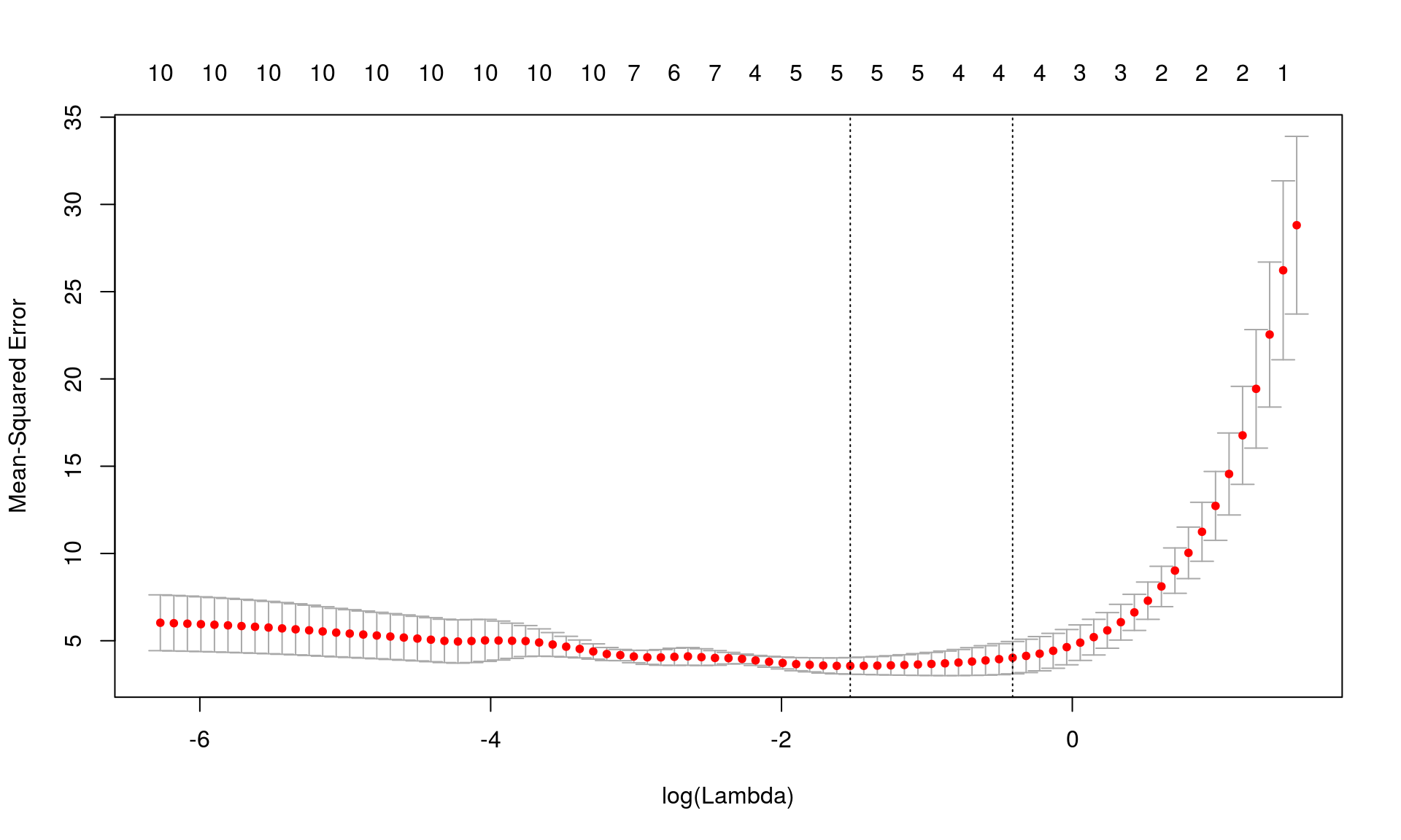
- The red dots are the average MSE over the k-folds.
- The two chosen \(\lambda\) values are the one with \(MSE_{min}\) and one with \(MSE_{min} + sd_{min}\)