The purr package

Package purrr is part of the tidyverse. Handles tasks similar to ones performed by apply-family functions in base R.

It enhances R’s functional programming toolkit by providing a complete and consistent set of tools for working with functions and vectors. map-functions allow you to replace many for loops with code that is easier to read.

• map(), map_if(), map_at() returns a list
• map_lgl() returns a logical vector,
• map_int() returns a integer vector,
• map_dbl() returns a double vector,
• map_chr() returns a character vector,
• map_dfr(), map_dfc() returns a data.frame
  by binding rows or columns respectively.

The map functions

Example: column-wise mean

df <- tibble(a=rnorm(10), b=rnorm(10), c=rnorm(10), d=rnorm(10))
map_dbl(df, mean)                       # or equivalently: df %>% map_dbl(mean)   

##          a          b          c          d 
## -0.1186649 -0.5658593  0.4204846 -0.1224230

Focus is on the operation being performed, not the book-keeping:

• purrr functions are implemented in C.
• the second argument, .f, can be a functions, a formula, a character vector, or an integer vector.

map(1:3, ~ rnorm(7, .x))

## [[1]]
## [1]  1.9179251 -0.2185906 -1.0120466  3.0876985  1.3292621  0.3024669
## [7]  1.0919825
## 
## [[2]]
## [1] 2.3569562 1.1267930 0.7098638 1.2323049 2.5096483 2.2123643 1.3248595
## 
## [[3]]
## [1] 3.555245 4.209644 2.563417 1.980601 3.985521 2.403396 3.056368

• map can pass additional parameters to the function

map_dbl(df, mean, trim = 0.25)

##          a          b          c          d 
##  0.1652477 -0.5862865  0.4144893 -0.1149048

• other inputs/outputs:

mtcars %>% 
  split(.$cyl)

## $`4`
##                 mpg cyl  disp  hp drat    wt  qsec vs am gear carb
## Datsun 710     22.8   4 108.0  93 3.85 2.320 18.61  1  1    4    1
## Merc 240D      24.4   4 146.7  62 3.69 3.190 20.00  1  0    4    2
## Merc 230       22.8   4 140.8  95 3.92 3.150 22.90  1  0    4    2
## Fiat 128       32.4   4  78.7  66 4.08 2.200 19.47  1  1    4    1
## Honda Civic    30.4   4  75.7  52 4.93 1.615 18.52  1  1    4    2
## Toyota Corolla 33.9   4  71.1  65 4.22 1.835 19.90  1  1    4    1
## Toyota Corona  21.5   4 120.1  97 3.70 2.465 20.01  1  0    3    1
## Fiat X1-9      27.3   4  79.0  66 4.08 1.935 18.90  1  1    4    1
## Porsche 914-2  26.0   4 120.3  91 4.43 2.140 16.70  0  1    5    2
## Lotus Europa   30.4   4  95.1 113 3.77 1.513 16.90  1  1    5    2
## Volvo 142E     21.4   4 121.0 109 4.11 2.780 18.60  1  1    4    2
## 
## $`6`
##                 mpg cyl  disp  hp drat    wt  qsec vs am gear carb
## Mazda RX4      21.0   6 160.0 110 3.90 2.620 16.46  0  1    4    4
## Mazda RX4 Wag  21.0   6 160.0 110 3.90 2.875 17.02  0  1    4    4
## Hornet 4 Drive 21.4   6 258.0 110 3.08 3.215 19.44  1  0    3    1
## Valiant        18.1   6 225.0 105 2.76 3.460 20.22  1  0    3    1
## Merc 280       19.2   6 167.6 123 3.92 3.440 18.30  1  0    4    4
## Merc 280C      17.8   6 167.6 123 3.92 3.440 18.90  1  0    4    4
## Ferrari Dino   19.7   6 145.0 175 3.62 2.770 15.50  0  1    5    6
## 
## $`8`
##                      mpg cyl  disp  hp drat    wt  qsec vs am gear carb
## Hornet Sportabout   18.7   8 360.0 175 3.15 3.440 17.02  0  0    3    2
## Duster 360          14.3   8 360.0 245 3.21 3.570 15.84  0  0    3    4
## Merc 450SE          16.4   8 275.8 180 3.07 4.070 17.40  0  0    3    3
## Merc 450SL          17.3   8 275.8 180 3.07 3.730 17.60  0  0    3    3
## Merc 450SLC         15.2   8 275.8 180 3.07 3.780 18.00  0  0    3    3
## Cadillac Fleetwood  10.4   8 472.0 205 2.93 5.250 17.98  0  0    3    4
## Lincoln Continental 10.4   8 460.0 215 3.00 5.424 17.82  0  0    3    4
## Chrysler Imperial   14.7   8 440.0 230 3.23 5.345 17.42  0  0    3    4
## Dodge Challenger    15.5   8 318.0 150 2.76 3.520 16.87  0  0    3    2
## AMC Javelin         15.2   8 304.0 150 3.15 3.435 17.30  0  0    3    2
## Camaro Z28          13.3   8 350.0 245 3.73 3.840 15.41  0  0    3    4
## Pontiac Firebird    19.2   8 400.0 175 3.08 3.845 17.05  0  0    3    2
## Ford Pantera L      15.8   8 351.0 264 4.22 3.170 14.50  0  1    5    4
## Maserati Bora       15.0   8 301.0 335 3.54 3.570 14.60  0  1    5    8

mtcars %>% 
  split(.$cyl) %>%
  map_df(dim)

## # A tibble: 2 x 3
##     `4`   `6`   `8`
##   <int> <int> <int>
## 1    11     7    14
## 2    11    11    11

Base-R maps vs. purrr maps

However, purrr is more consistent, so you should learn it.

A quick reference of similar base R functions:

• lapply is basically identical to map

• sapply is a wrapper around lapply and it tries to simplify the output. Downside: you never know what you’ll get

• vapply: like sapply, but you can supply an additional argument that defines the type

You can learn more about purr here: (http://r4ds.had.co.nz/iteration.html)

Missing values

Two types of missingness

stocks <- tibble(
  year   = c(2015, 2015, 2015, 2015, 2016, 2016, 2016),
  qtr    = c(   1,    2,    3,    4,    2,    3,    4),
  return = c(1.88, 0.59, 0.35,   NA, 0.92, 0.17, 2.66)
)

The return for the fourth quarter of 2015 is explicitly missing

The return for the first quarter of 2016 is implicitly missing

The way that a dataset is represented can make implicit values explicit.

stocks %>% spread(year, return)

## # A tibble: 4 x 3
##     qtr `2015` `2016`
##   <dbl>  <dbl>  <dbl>
## 1     1   1.88  NA   
## 2     2   0.59   0.92
## 3     3   0.35   0.17
## 4     4  NA      2.66

Gathering missing data

Recall the functions we learned from tidyr package.

You can used spread() and gather() to retain only non-missing recored, i.e. to turn all explicit missing values into implicit ones.

stocks %>% spread(year, return) %>% 
  gather(year, return, `2015`:`2016`, na.rm = TRUE)

## # A tibble: 6 x 3
##     qtr year  return
## * <dbl> <chr>  <dbl>
## 1     1 2015    1.88
## 2     2 2015    0.59
## 3     3 2015    0.35
## 4     2 2016    0.92
## 5     3 2016    0.17
## 6     4 2016    2.66

Completing missing data

complete() takes a set of columns, and finds all unique combinations. It then ensures the original dataset contains all those values, filling in explicit NAs where necessary.

stocks %>% complete(year, qtr)

## # A tibble: 8 x 3
##    year   qtr return
##   <dbl> <dbl>  <dbl>
## 1  2015     1   1.88
## 2  2015     2   0.59
## 3  2015     3   0.35
## 4  2015     4  NA   
## 5  2016     1  NA   
## 6  2016     2   0.92
## 7  2016     3   0.17
## 8  2016     4   2.66

Different intepretations of NA

Sometimes when a data source has primarily been used for data entry, missing values indicate that the previous value should be carried forward:

# tribble() constructs a tibble by filling by rows
treatment <- tribble(
  ~ person,           ~ treatment, ~response,
  "Derrick Whitmore", 1,           7,
  NA,                 2,           10,
  NA,                 3,           9,
  "Katherine Burke",  1,           4
)

You can fill in these missing values with fill()

treatment %>% fill(person)

## # A tibble: 4 x 3
##   person           treatment response
##   <chr>                <dbl>    <dbl>
## 1 Derrick Whitmore         1        7
## 2 Derrick Whitmore         2       10
## 3 Derrick Whitmore         3        9
## 4 Katherine Burke          1        4

Relational data

• Rarely does a data analysis involve only a single table of data.

• Collectively, multiple tables of data are called relational data because the relations, not just the individual datasets, that are important.

• Relations are always defined between a pair of tables.

• All other relations are built up from this simple idea: the relations of three or more tables are always a property of the relations between each pair.

Example

the nycflights13 package contains a collection of related datasets.

library(nycflights13)

Source: (http://r4ds.had.co.nz/relational-data.html)

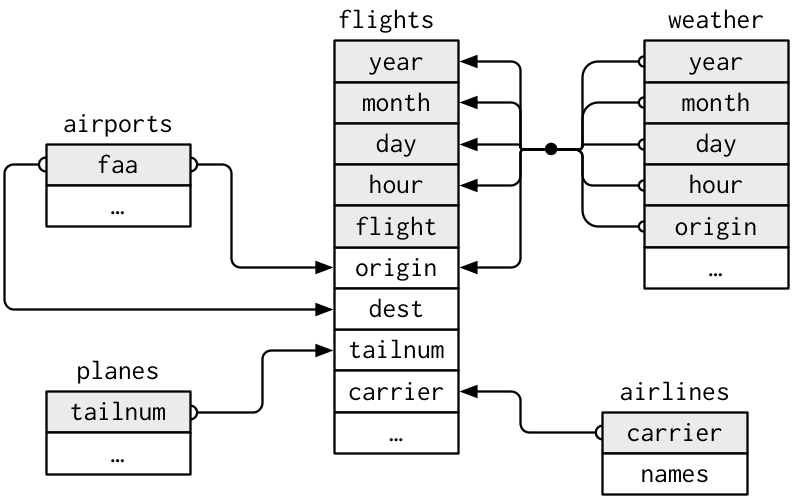
Keys

A key is a variable (or set of variables) that uniquely identifies an observation.

For example, each plane is uniquely determined by its tailnum, but an observation in ‘weather’ is identified by five variables: year, month, day, hour, and origin

Keys can be used to connect each pair of tables together.

There are two types of keys:

• Primary: identifies an observation in its own table. Example: planes$tailnum

• Foreign: identifies an observation in another table. Example: flights$tailnum, this is because tailnum does not enough to identify a record in flights dataset.

A variable can be both a primary key and a foreign key.

Identify primary keys

It’s good practice to verify that chosen keys do indeed uniquely identify each observation.

One way to do that is to count() the primary keys and look for entries where n is greater than one:

planes %>% 
  count(tailnum) %>% 
  filter(n > 1)

## # A tibble: 0 x 2
## # ... with 2 variables: tailnum <chr>, n <int>

weather %>% 
  count(year, month, day, hour, origin) %>% 
  filter(n > 1)

## # A tibble: 3 x 6
##    year month   day  hour origin     n
##   <dbl> <dbl> <int> <int> <chr>  <int>
## 1  2013    11     3     1 EWR        2
## 2  2013    11     3     1 JFK        2
## 3  2013    11     3     1 LGA        2

No primary key

Sometimes a table doesn’t have an explicit primary key, e.g. in flights dataset each row is an observation, but no combination of variables reliably identifies it, (even the flight numbers).

In this case, you can add an extra identifier column:

flights %>% 
  count(flight) %>% 
  filter(n > 1) 

## # A tibble: 3,493 x 2
##    flight     n
##     <int> <int>
##  1      1   701
##  2      2    51
##  3      3   631
##  4      4   393
##  5      5   324
##  6      6   210
##  7      7   237
##  8      8   236
##  9      9   153
## 10     10    61
## # ... with 3,483 more rows

flights %>%
  mutate(flight_id= paste0("F", row_number())) %>%
  select(flight_id, year:flight)

## # A tibble: 336,776 x 12
##    flight_id  year month   day dep_time sched_dep_time dep_delay arr_time
##    <chr>     <int> <int> <int>    <int>          <int>     <dbl>    <int>
##  1 F1         2013     1     1      517            515         2      830
##  2 F2         2013     1     1      533            529         4      850
##  3 F3         2013     1     1      542            540         2      923
##  4 F4         2013     1     1      544            545        -1     1004
##  5 F5         2013     1     1      554            600        -6      812
##  6 F6         2013     1     1      554            558        -4      740
##  7 F7         2013     1     1      555            600        -5      913
##  8 F8         2013     1     1      557            600        -3      709
##  9 F9         2013     1     1      557            600        -3      838
## 10 F10        2013     1     1      558            600        -2      753
## # ... with 336,766 more rows, and 4 more variables: sched_arr_time <int>,
## #   arr_delay <dbl>, carrier <chr>, flight <int>

Merging two tables

There are three families of functions designed to merge relational data:

• Mutating joins, which add new variables to one data frame from matching observations in another.

• Filtering joins, which filter observations from one data frame based on whether or not they match an observation in the other table.

• Set operations, which treat observations as if they were set elements.

Mutating joins

A mutating join allows you to combine variables from two tables, by matching observations by their keys, and then copying across variables from one table to the other. e.g.

flights %>%
  select(year:day, hour, origin, dest, tailnum, carrier) %>% 
  left_join(airlines, by = "carrier")

## # A tibble: 336,776 x 9
##     year month   day  hour origin dest  tailnum carrier name              
##    <int> <int> <int> <dbl> <chr>  <chr> <chr>   <chr>   <chr>             
##  1  2013     1     1     5 EWR    IAH   N14228  UA      United Air Lines …
##  2  2013     1     1     5 LGA    IAH   N24211  UA      United Air Lines …
##  3  2013     1     1     5 JFK    MIA   N619AA  AA      American Airlines…
##  4  2013     1     1     5 JFK    BQN   N804JB  B6      JetBlue Airways   
##  5  2013     1     1     6 LGA    ATL   N668DN  DL      Delta Air Lines I…
##  6  2013     1     1     5 EWR    ORD   N39463  UA      United Air Lines …
##  7  2013     1     1     6 EWR    FLL   N516JB  B6      JetBlue Airways   
##  8  2013     1     1     6 LGA    IAD   N829AS  EV      ExpressJet Airlin…
##  9  2013     1     1     6 JFK    MCO   N593JB  B6      JetBlue Airways   
## 10  2013     1     1     6 LGA    ORD   N3ALAA  AA      American Airlines…
## # ... with 336,766 more rows

Mutating joins

There are four mutating join functions:

• inner_join()

• outer joins;
  • left_join()
  • right_join()
  • full_join()

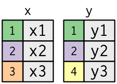
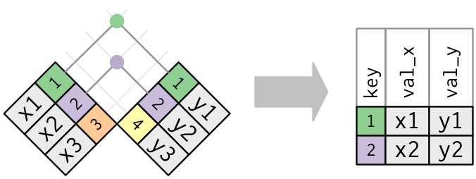
A simple example

x <- tribble(
  ~key, ~val_x,
     1, "x1",
     2, "x2",
     3, "x3"
)

y <- tribble(
  ~key, ~val_y,
     1, "y1",
     2, "y2",
     4, "y3"
)

Inner join

x %>% inner_join(y, by = "key")

## # A tibble: 2 x 3
##     key val_x val_y
##   <dbl> <chr> <chr>
## 1     1 x1    y1   
## 2     2 x2    y2

Source: (http://r4ds.had.co.nz/relational-data.html)

Outer join

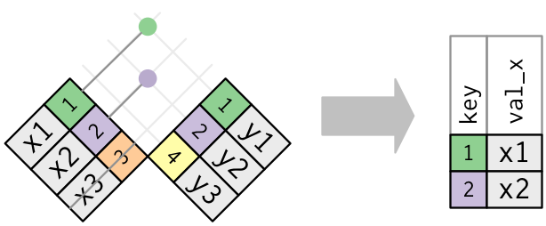
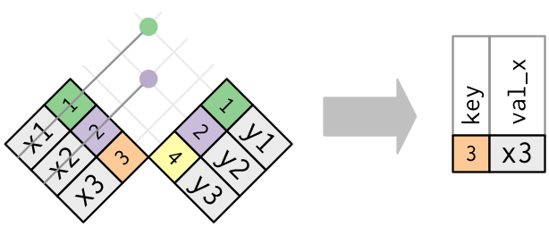
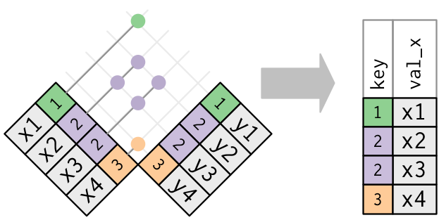
Duplicate keys

What happens when there are duplicate keys?

• One table has duplicate keys. There may be a one-to-many relation.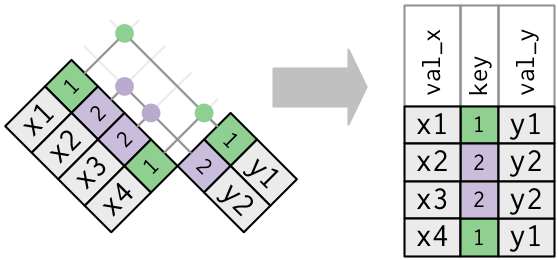

• Both tables have duplicate keys. When you join duplicated keys, you get all possible combinations: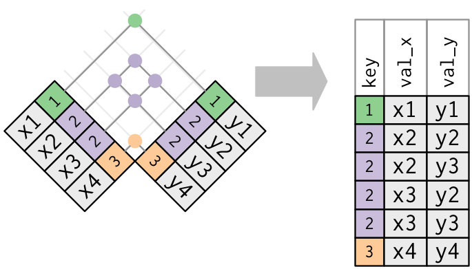

Source: http://r4ds.had.co.nz/relational-data.html

Filtering joins

Filtering joins match observations in the same way as mutating joins, but affect the observations, not the variables.

There are two types:

• semi_join(x, y) keeps all observations in x that have a match in y.
• anti_join(x, y) drops all observations in x that have a match in y.

Multiple matches

In filtering joins, only the existence of a match is important.

It doesn’t matter which observation is matched.

Filtering joins never duplicate rows like mutating joins do:

Set operations

Set operations apply to rows; they expect the x and y inputs to have the same variables, and treat the observations like sets.

• intersect(x, y): returns only observations in both x and y.

• union(x, y): returns unique observations in x and y.

• setdiff(x, y): returns observations in x, but not in y.

All these operations work with a complete row, comparing the values of every variable.

Example

df1 <- tribble(
  ~x, ~y,
   1,  1,
   2,  1
)
df2 <- tribble(
  ~x, ~y,
   1,  1,
   1,  2
)

intersect(df1, df2)

## # A tibble: 1 x 2
##       x     y
##   <dbl> <dbl>
## 1     1     1

union(df1, df2)

## # A tibble: 3 x 2
##       x     y
##   <dbl> <dbl>
## 1     1     2
## 2     2     1
## 3     1     1

setdiff(df1, df2)

## # A tibble: 1 x 2
##       x     y
##   <dbl> <dbl>
## 1     2     1

setdiff(df2, df1)

## # A tibble: 1 x 2
##       x     y
##   <dbl> <dbl>
## 1     1     2

Exporting Data

After working with a dataset and doing all data manipulation, you might want to save your new data table.

Recall the readr package. Besides functions for reading data in, readr has utilities for saving your data to a text file:

write_tsv(mydata, "path/to/filename.tsv")                  # tab-delimited
write_csv(mydata, "path/to/filename.csv")                  # comma-delimited
write_delim(mydata, "path/to/filename.csv", delim = " ")   # general delimiter

To save your data in other types of files, you need to install and use other packages:

• to export an Excel spreadsheet, use xlsx package, and follow this guide.

# install.packages(xlsx)
library(xlsx)
write.xlsx(mydata, "path/to/filename.xlsx")

• to export SAS, SPSS and Stata files use the haven package.

# install.packages(haven)
library(haven)
read_sas("mtcars.sas7bdat")
write_sas(mtcars, "mtcars.sas7bdat")

Saving the workspace

• You can also choose to save all objects currently in the workspace (variables, functions, etc.) into a file e.g. filename.rda.

• The file filename.rda can be the easily loaded next time you work with R.

• You can also save a single object or a subset of specified objects currently in the workspace.

# save the workspace to file 
save.image(file = "path/to/filename.rda")

# save specific objects to a file
save(object_list, file = "path/to/filename.rda")

# save just a single object
saveRDS(object, file = "path/to/filename.rds")

• Saved objects/workspace can be loaded back in a new R session.

# load a workspace into the current session
load("path/to/filename.rda")

# read just the previously saved 1 object
object <- readRDS("path/to/filename.rds")

Exercise 1

• Go to “Lec5_Exercises.Rmd” on the class website.

• Complete Exercise 1.

What is exploratory data analysis (EDA)?

There are no routine statistical questions, only questionable statistical routines.  — Sir David Cox

EDA is an iterative process:

• Generate questions about your data
• Search for answers by visualising, transforming, and modelling data

Use what you learn to refine your questions or generate new ones.

Asking questions

Your goal during EDA is to develop an understanding of your data.

EDA is fundamentally a creative process. And like most creative processes, the key to asking quality questions is to generate a large quantity of questions.¹

Two types of questions will always be useful for making discoveries within your data:

1. What type of variation occurs within my variables?
2. What type of covariation occurs between my variables?

Some comments about EDA:

• It is not a formal process with a strict set of rules.
• Explore many ideas: some will pan out, others will be dead ends.
• Even if questions are predefined, quality of data still needs to be assessed

Variation

Variation is the tendency of the values of a variable to change from measurement to measurement. Every variable has its own pattern of variation, which can reveal interesting information.²

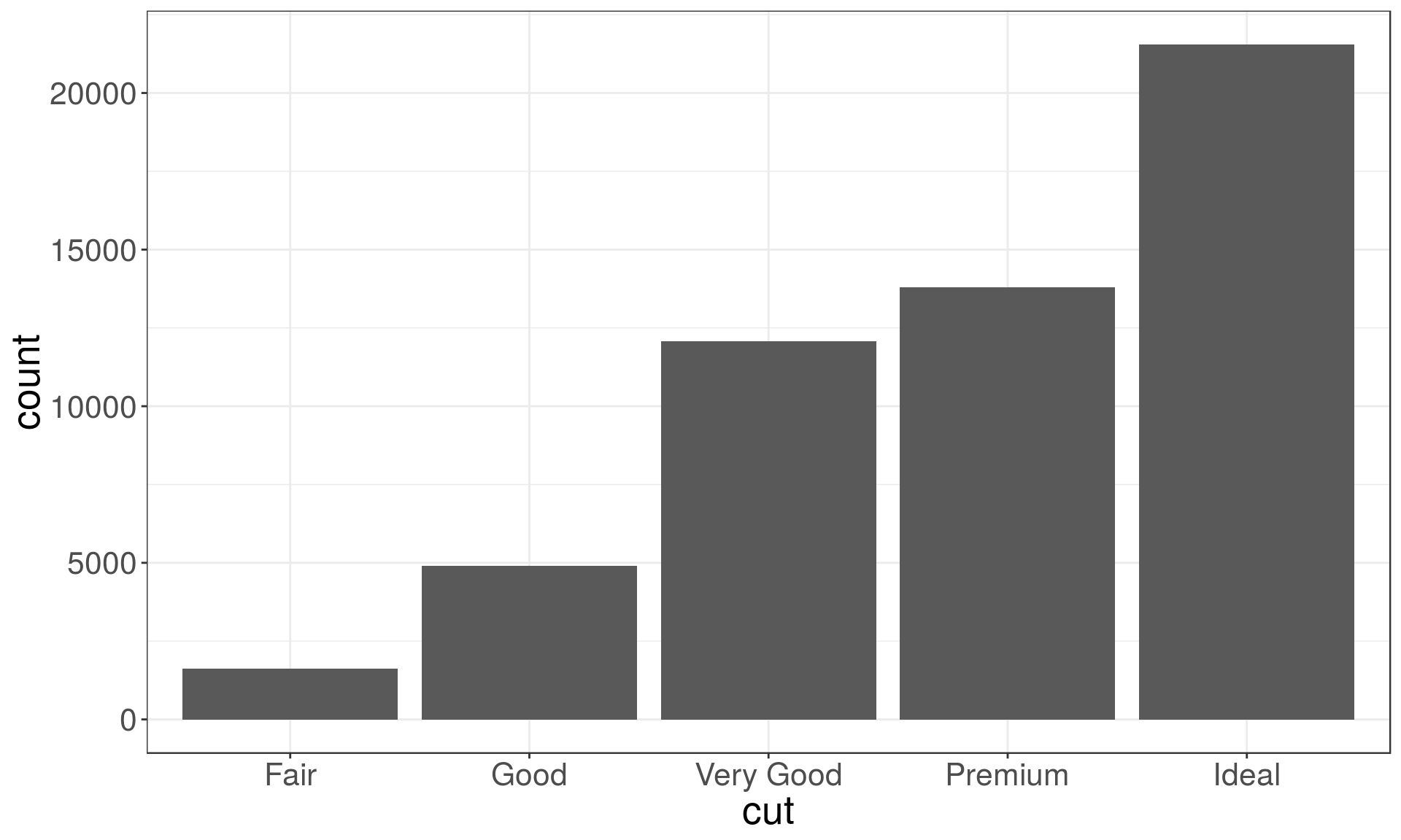
Recall the diamonds dataset. Use a bar chart, to examine the distribution of a categorical variable, and a histogram that of a continuous one.

ggplot(data = diamonds) +
  geom_bar(mapping = aes(x = cut))

ggplot(data = diamonds) +
  geom_histogram(mapping = aes(x = carat), binwidth = 0.5)

Identifying typical values

• Which values are the most common? Why?
• Which values are rare? Why? Does that match your expectations?
• Can you see any unusual patterns? What might explain them?

diamonds %>% filter(carat < 3) %>%
  ggplot(aes(x = carat)) + geom_histogram(binwidth = 0.01)

Look for anything unexpected!

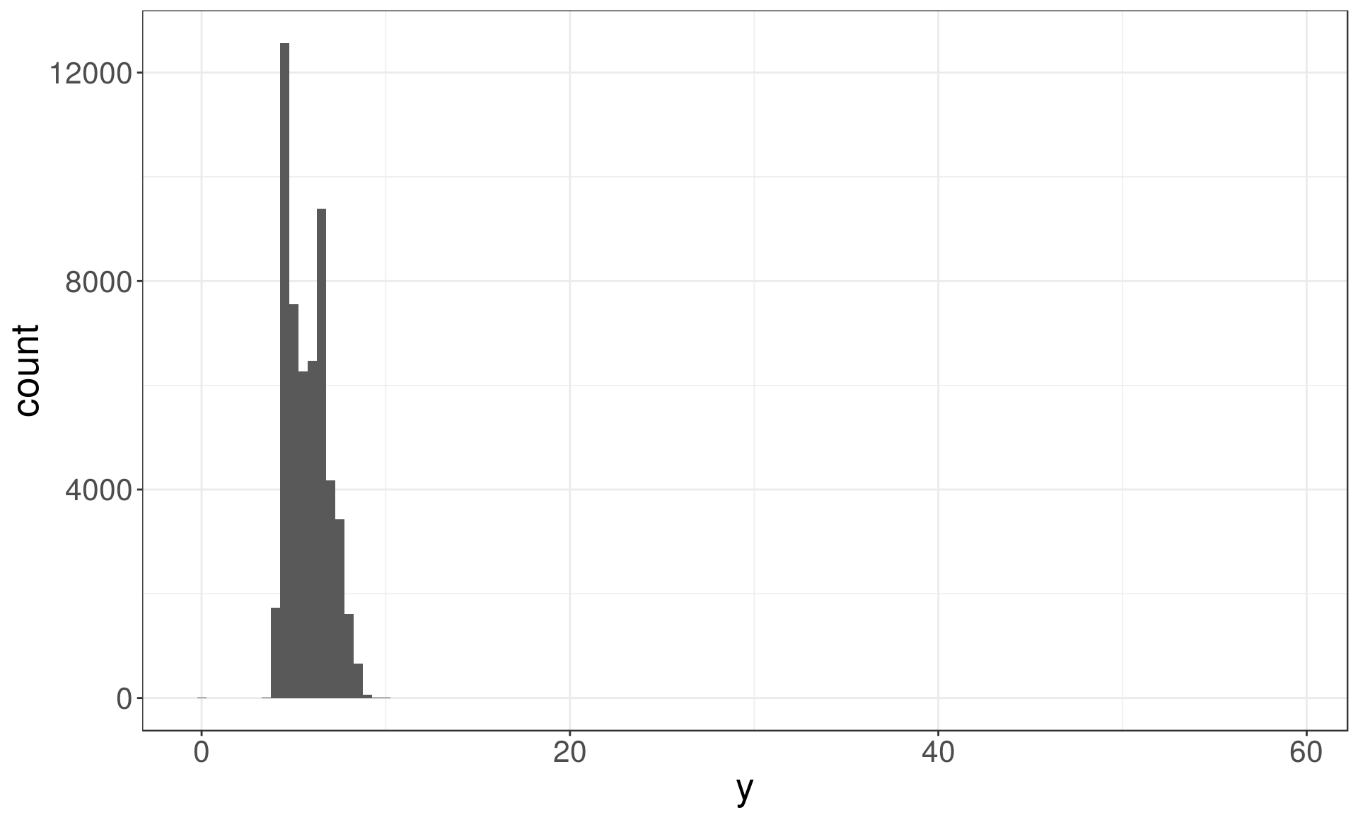
Identify outliers

Outliers are observations that are unusual – data points that don’t seem to fit the general pattern.

Sometimes outliers are data entry errors; other times outliers suggest important new science.

ggplot(diamonds) + 
  geom_histogram(mapping = aes(x = y), binwidth = 0.5)

ggplot(diamonds) + 
  geom_histogram(mapping = aes(x = y), binwidth = 0.5) +
  coord_cartesian(ylim = c(0, 50))

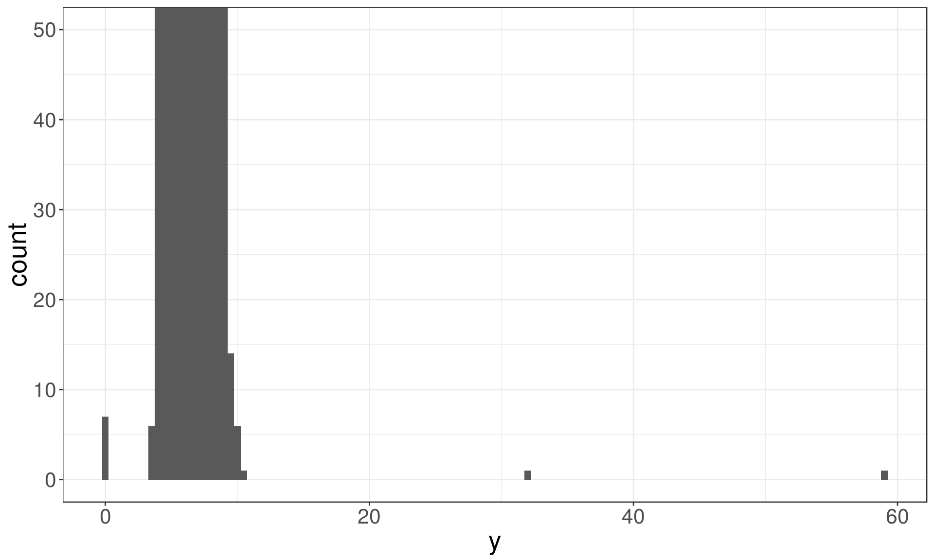
Identifying outliers

Now that we have seen the usual values, we can try to understand them.

diamonds %>% filter(y < 3 | y > 20) %>% 
  select(price, carat, x, y, z) %>% arrange(y)

## # A tibble: 9 x 5
##   price carat     x     y     z
##   <int> <dbl> <dbl> <dbl> <dbl>
## 1  5139  1     0      0    0   
## 2  6381  1.14  0      0    0   
## 3 12800  1.56  0      0    0   
## 4 15686  1.2   0      0    0   
## 5 18034  2.25  0      0    0   
## 6  2130  0.71  0      0    0   
## 7  2130  0.71  0      0    0   
## 8  2075  0.51  5.15  31.8  5.12
## 9 12210  2     8.09  58.9  8.06

The y variable measures the length (in mm) of one of the three dimensions of a diamond.

Therefore, these must be entry errors! Why?

It’s good practice to repeat your analysis with and without the outliers.

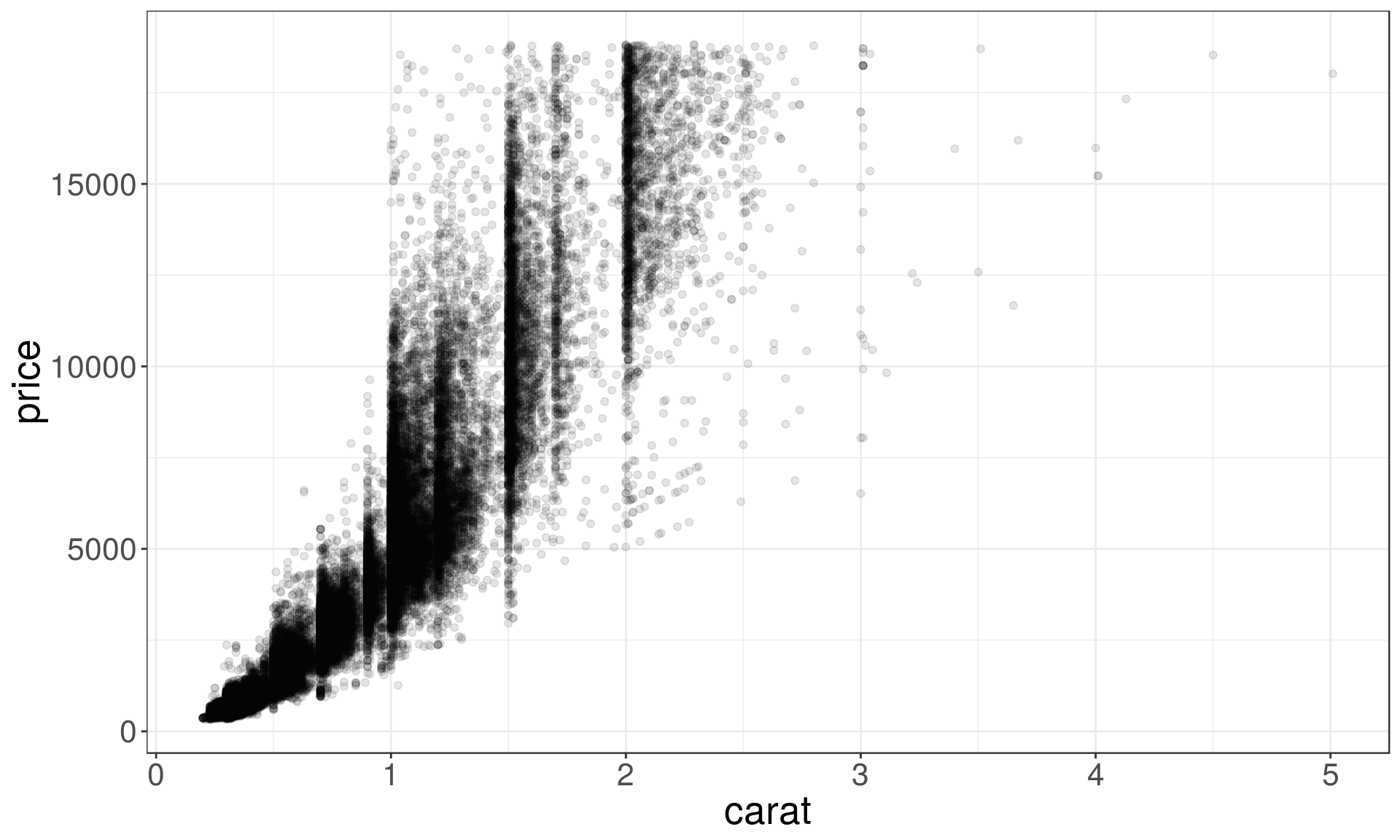
Covariation

Covariation is the tendency for the values of two or more variables to vary together in a related way.

ggplot(data = diamonds) + 
  geom_point(aes(x=carat, y=price), alpha=0.1) 

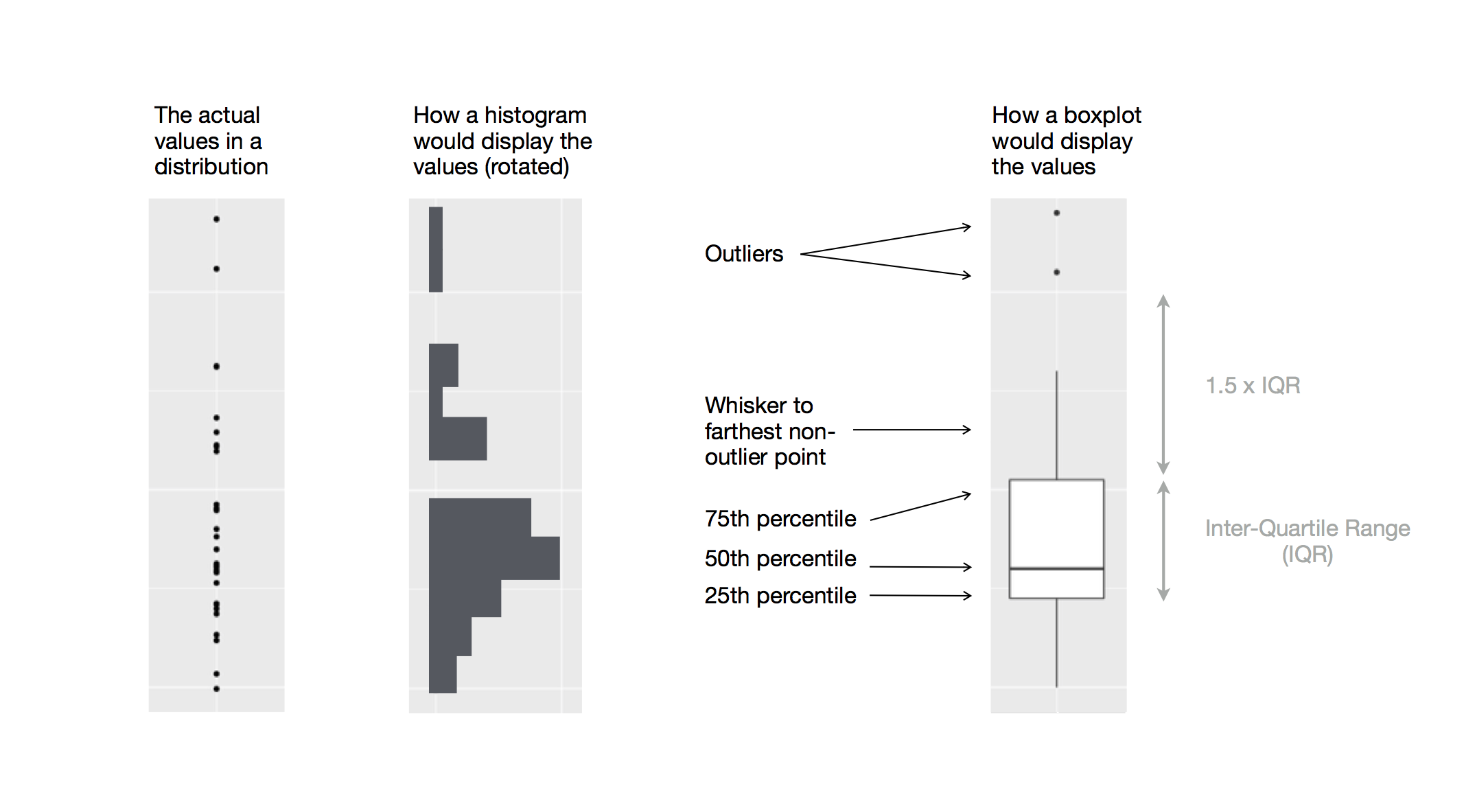
Boxplots

Boxplot are used to display visual shorthand for a distribution of a continuous variable broken down by categories.

They mark the distribution’s quartiles.

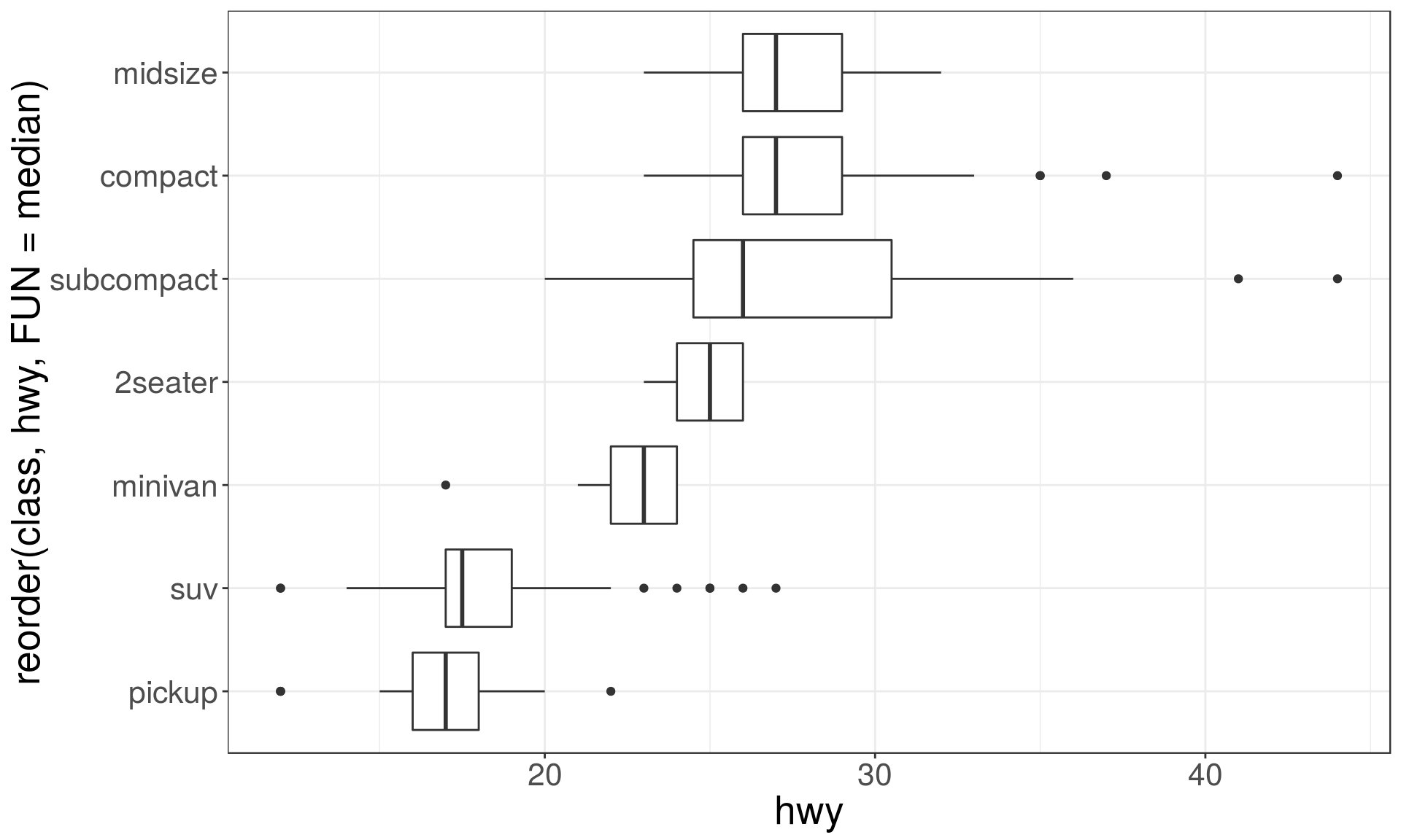
A categorical and a continuous variable

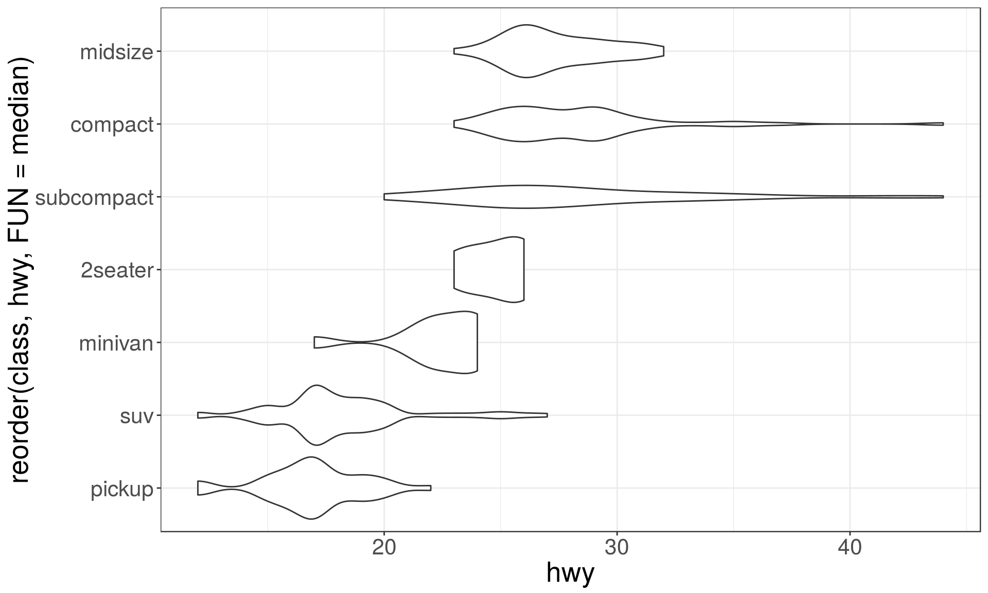
Use a boxplot or a violin plot to display the covariation between a categorical and a continuous variable.

Violin plots give more information, as they show the entrire estimated distribution.

ggplot(mpg, aes(
  x = reorder(class, hwy, FUN = median), y = hwy)) +
  geom_boxplot() + coord_flip()

ggplot(mpg, aes(
  x = reorder(class, hwy, FUN = median), y = hwy)) +
  geom_violin() + coord_flip()

Two categorical variables

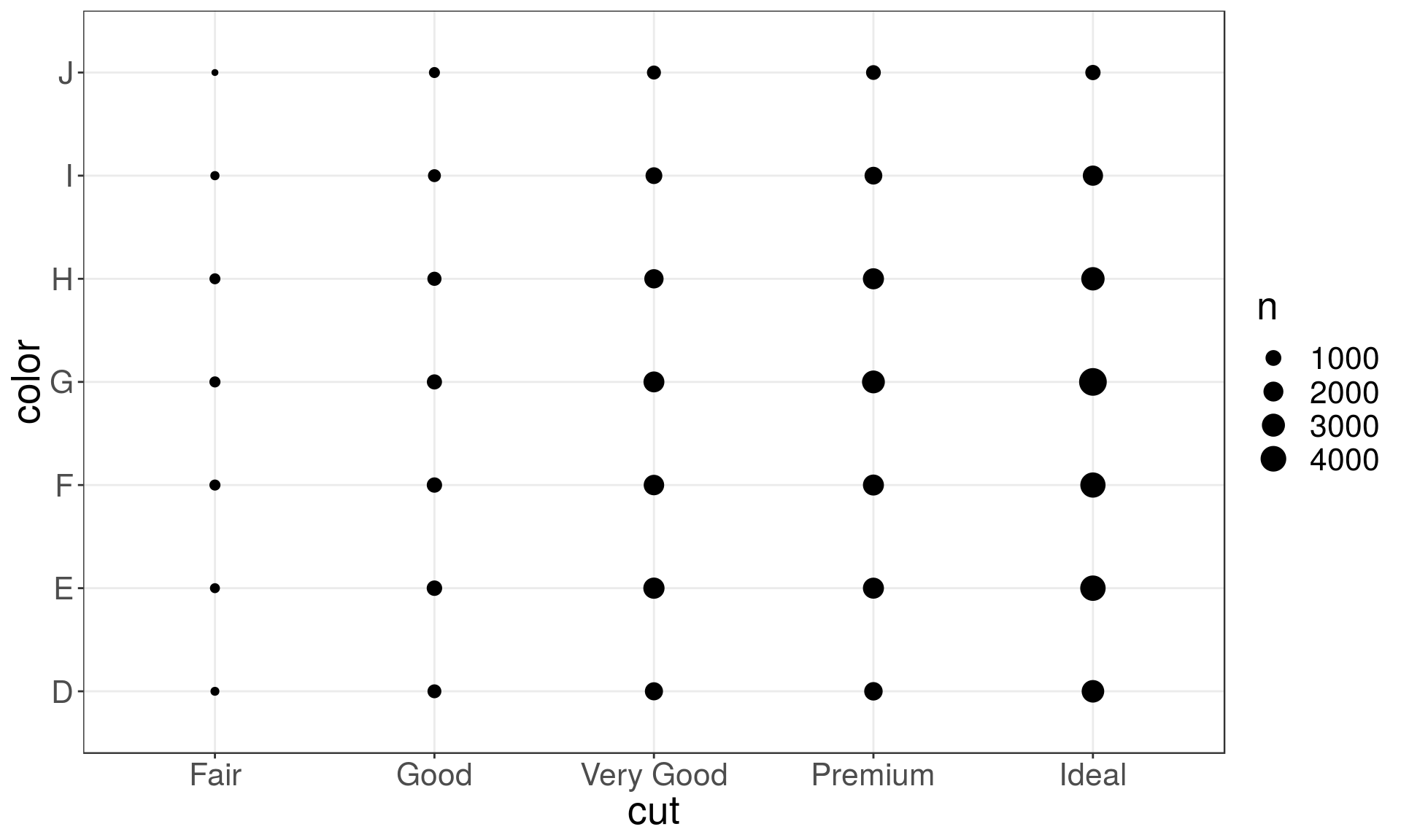
To visualise the covariation between categorical variables, you need to count the number of observations for each combination, e.g. using geom_count():

ggplot(data = diamonds) +
  geom_count(mapping = aes(x = cut, y = color))

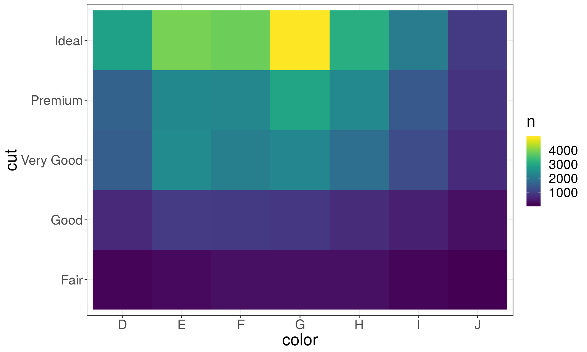
Another approach is to first, compute the count and then visualise it by coloring with geom_tile() and the fill aesthetic:

diamonds %>% 
  count(color, cut) %>%  
  ggplot(mapping = aes(x = color, y = cut)) +
    geom_tile(mapping = aes(fill = n)) +
  scale_fill_viridis()

Two continuous variables

ggplot(data = diamonds) +
  geom_point(mapping = aes(x = carat, y = price)) + 
  scale_y_log10() + scale_x_log10() 

# install.packages("hexbin")
ggplot(data = diamonds) +
  geom_hex(mapping = aes(x = carat, y = price)) +
  scale_y_log10() + scale_x_log10() 

Exercise 2

• Go to “Lec5_Exercises.Rmd” on the class website.

• Complete Exercise 2.

The plotly package

• plotly is a package for visualization and a collaboration platform for data science
• Available in R, python, MATLAB, scala.
  
• You can produce interactive graphics including 3D plots (with zooming and rotating).
• You can open a ‘plotly’ account to upload ‘plotly’ graphs and view or modify them in a web browser.
• Resources: cheatsheet, book

plotly integration with ggplot2

library(plotly); library(tidyverse) # or library(ggplot2); library(dplyr)
plt <- ggplot(diamonds %>% sample_n(1000), aes(x = carat, y = price)) + 
  geom_point(aes(color = cut))
ggplotly(plt) 

plt <- ggplot(diamonds %>% sample_n(1000), aes(x = carat, y = price)) + 
  geom_text(aes(label = clarity), size = 4) + 
  geom_smooth(aes(color = cut, fill = cut)) +
  facet_wrap(~cut)
ggplotly(plt) 

## `geom_smooth()` using method = 'loess' and formula 'y ~ x'

3D Scatter plots

theta <- seq(0, 10, 0.2); 
df <- data.frame(U = theta, V =  cos(theta), W = sin(theta)*theta)
plot_ly(df, x = ~V, y = ~W, z = ~U, type = "scatter3d", mode = "markers",
        marker = list(size = 3))

Adding layers

dbl.helix <- data.frame(t = rep(seq(0, 2*pi, length.out = 100), 3)) %>%
  mutate(x1 = sin(t), y1 = cos(t), z = (1:length(t))/10,
         x2 = sin(t + pi/2), y2 = cos(t + pi/2))
plot_ly(dbl.helix, x = ~x1, y = ~y1, z = ~z, type = "scatter3d", mode = "lines", 
        color = "green", colors = c("green", "purple"), line = list(width = 5)) %>% 
  add_trace(x = ~x2, y = ~y2, z = ~z+0.2, color = "purple") 

Volcano dataset

• volcano - a built-in dataset storing topographic information for Maunga Whau (Mt Eden), one of 50 volcanos in Auckland, New Zealand.
• It consist of a 87 x 61 matrix with entries corresponding to the mountain’s atlitutes [m] on a 10m by 10m grid.
  
• rows run east to west, and columns south to north

dim(volcano)

## [1] 87 61

volcano[1:5, 1:5]

##      [,1] [,2] [,3] [,4] [,5]
## [1,]  100  100  101  101  101
## [2,]  101  101  102  102  102
## [3,]  102  102  103  103  103
## [4,]  103  103  104  104  104
## [5,]  104  104  105  105  105

2D contour plots

plot_ly(z = volcano) %>% add_contour()

3D surface plots

plot_ly(z = volcano) %>% add_surface()

Exercise 3

• Go to “Lec5_Exercises.Rmd” on the class website.

• Complete Exercise 3.