Lecture 3: Importing and transforming data

CME/STATS 195

Lan Huong Nguyen

October 4, 2018

Importing data
Tidying data
Transforming data
Chaining operations

Importing data

Working Directory

The current working directory (cmd) is the location which R is currently pointing to.
Whenever you try to read or save a file without specifying the path explicitly, the cmd will be used by default.
When are executing code from an R markdown/notebook code chunk, the cmd is the location of the document.
To see the current working directory use getwd():

getwd()   # with no arguments

## [1] "/home/lanhuong/MEGA/Teaching/cme195_intro_to_R/cme195.github.io/assets/lectures"

To change the working directory use setwd(path_name) with a specified path as na argument:

setwd("path/to/directory")

Paths and directory names

R inherits its file and folder naming conventions from unix, and uses forward slashes for the directories, e.g. /home/lan/folder/
This is, because backslashes serve a different purpose; they are used as escape characters to isolate special characters and stop them from being immediately interpreted.
When working with R on Windows, you can use either: C:/Path/To/A/File or C:\\Path\\To\\A\\File
Use a “Tab” for autocompletion to find file paths more easily.
To avoid problems, directory names should NOT contain spaces and special characters.

Importing text data

Text Files in a table format can be read and saved to a selected variable using a read.table() function. Use ?read.table to learn more about the function.
A common text file format is a comma delimited text file, .csv. These files use a comma as column separators, e.g:

Year,Student,Major
2009, John Doe,Statistics
2009, Bart Simpson, Mathematics I

To read these files use the following command:

mydata <- read.table("path/to/filename.csv", header=TRUE,  sep = ",")

# read.csv() has covenient argument defaults for '.csv' files
mydata <- read.csv("path/to/filename.csv")

Optionally, use row.names or col.names arguments to set the row and column names.

The `readr` package

Many R packages provide examples of data. However, sooner or later you will need to work with your own data.

readr is for reading rectangular text data into R.

readr supports several file formats with seven read_<...> functions:

read_csv(): comma-separated (CSV) files
read_tsv(): tab-separated files
read_delim(): general delimited files
read_fwf(): fixed-width files
read_table(): tabular files where colums are separated by white-space
read_log(): web log files

In many cases it just works: supply path to a file and get a tibble back.

Comparison with base R

Why are we learning the readr package?

it is up to 10x faster
it produces tibbles instead of data.frames
better parsing (e.g. does not convert strings to factors)
more reproducible on different systems
progress bar for large files

Reading comma-separated files

All read_<...>() functions have a similar syntax, so we focus on read_csv().

# Get path to example dataset
readr_example("mtcars.csv")

## [1] "/home/lanhuong/R/x86_64-pc-linux-gnu-library/3.4/readr/extdata/mtcars.csv"

mtcars <- read_csv(readr_example("mtcars.csv"))

## Parsed with column specification:
## cols(
##   mpg = col_double(),
##   cyl = col_integer(),
##   disp = col_double(),
##   hp = col_integer(),
##   drat = col_double(),
##   wt = col_double(),
##   qsec = col_double(),
##   vs = col_integer(),
##   am = col_integer(),
##   gear = col_integer(),
##   carb = col_integer()
## )

mtcars is a dataset on fuel consumption, and other 10 aspects of design and performance (?mtcars).

The `read_csv()` function

Also works with inline csv files (useful for experimenting).

read_csv(
  "a,b,c
  1,2,3
  4,5,6"
)

## # A tibble: 2 x 3
##       a     b     c
##   <int> <int> <int>
## 1     1     2     3
## 2     4     5     6

read_csv(
  "a,b,c
  1,2,3
  4,5,6", 
  col_names=FALSE
)

## # A tibble: 3 x 3
##   X1    X2    X3   
##   <chr> <chr> <chr>
## 1 a     b     c    
## 2 1     2     3    
## 3 4     5     6

Other useful arguments: skip lines, symbol for missing data.

Now you can read most CSV files, also easily adapt to read_tsv(),
read_fwf(). For the others, you need to know how readr works inside.

How `readr` parses data?

parse_logical(c("TRUE","FALSE"))

## [1]  TRUE FALSE

parse_integer(c("1","2","3","NA"))

## [1]  1  2  3 NA

Parsing vectors:

parse_logical(), parse_integer()
parse_double(), parse_number(): for numbers from other countries
parse_character(): for character encodings.
parse_datetime(), parse_date(), parse_time()
parse_factor()

Potential difficulties

Parsing data is not always trivial:

Numbers are written differently in different parts of the world (“,” vs “.” for separatimg thousands)
Numbers are often surrounded by other characters (“$1000”, “10%”)
Numbers often contain “grouping” characters (“1,000,000”)
There are many different ways of writing dates and times
Times can be in different timezones
Encodings: special characters in other languages

Locales

A locale specifies common options varying between languages and places

To create a new locale, you use the locale() function:

locale(
  date_names = "en", 
  date_format = "%AD", 
  time_format = "%AT",
  decimal_mark = ".", 
  grouping_mark = ",", 
  tz = "UTC",
  encoding = "UTF-8", 
  asciify = FALSE)

## <locale>
## Numbers:  123,456.78
## Formats:  %AD / %AT
## Timezone: UTC
## Encoding: UTF-8
## <date_names>
## Days:   Sunday (Sun), Monday (Mon), Tuesday (Tue), Wednesday (Wed), Thursday
##         (Thu), Friday (Fri), Saturday (Sat)
## Months: January (Jan), February (Feb), March (Mar), April (Apr), May (May),
##         June (Jun), July (Jul), August (Aug), September (Sep), October
##         (Oct), November (Nov), December (Dec)
## AM/PM:  AM/PM

# More on locales can be found in a vignette
vignette("locales")

Parsing dates

parse_date() expects a four digit year, month, day separated by “-” or “/”:

parse_date("2010-10-01")

## [1] "2010-10-01"

Example: French format with full name of month:

parse_date("1 janvier 2010")

## Warning: 1 parsing failure.
## row # A tibble: 1 x 4 col     row   col expected     actual         expected   <int> <int> <chr>        <chr>          actual 1     1    NA "date like " 1 janvier 2010

## [1] NA

parse_date("1 janvier 2010", format="%d %B %Y", locale=locale("fr"))

## [1] "2010-01-01"

Learn more by typing ?parse_date

Parsing times

parse_time() expects an “hour : minutes” pair
(optionally proceeded by “:seconds”, and “am/pm” specifier).

parse_time("01:10 am")

## 01:10:00

Parsing dates and times:

parse_datetime("2001-10-10 20:10", locale = locale(tz = "Europe/Dublin"))

## [1] "2001-10-10 20:10:00 IST"

For more details, see the book R for data science or use the documentation.

Parsing numbers

parse_number() ignores non-numeric characters before and after.

parse_number("20%")

## [1] 20

parse_number("$100")

## [1] 100

parse_number("cost: $123.45")

## [1] 123.45

Parsing numbers with locales

# Separation used in Switzerland
parse_number("123'456'789", locale = locale(grouping_mark = "'"))

## [1] 123456789

Parsing real numbers

Real numbers using a different decimal mark

parse_double("1,23")

## Warning: 1 parsing failure.
## row # A tibble: 1 x 4 col     row   col expected               actual expected   <int> <int> <chr>                  <chr>  actual 1     1    NA no trailing characters ,23

## [1] NA
## attr(,"problems")
## # A tibble: 1 x 4
##     row   col expected               actual
##   <int> <int> <chr>                  <chr> 
## 1     1    NA no trailing characters ,23

parse_double("1,23", locale = locale(decimal_mark = ","))

## [1] 1.23

`readr’s` strategy for parsing files

readr uses a heuristic to determine column type, using the first 1000 rows.

You can emulate this process with two functions:

guess_parser(): returns readr’s best guess
parse_guess(): uses that guess to parse the column

The heuristic tries a sequence of types, stopping when it finds a match.

If none of these rules apply, then the column will stay as a vector of strings.

guess_parser("15:01")

## [1] "time"

guess_parser("Oct 10, 2010; 15:01")

## [1] "character"

parse_guess("12,352,561")

## [1] 12352561

parse_guess(c("TRUE", "FALSE"))

## [1]  TRUE FALSE

When the default strategy fails

The default strategy does not always work, e.g. if the first 1000 rows might be a special case. Suppose, your dataset with two columns:

# Top 1000 lines are (integer, missing)
readLines(readr_example("challenge.csv"), 10)

##  [1] "x,y"     "404,NA"  "4172,NA" "3004,NA" "787,NA"  "37,NA"   "2332,NA"
##  [8] "2489,NA" "1449,NA" "3665,NA"

# The remaining are (real number, date)
tail(readLines(readr_example("challenge.csv"), 3000), 4)

## [1] "0.47193897631950676,2014-08-04" "0.7183186465408653,2015-08-16" 
## [3] "0.26987858884967864,2020-02-04" "0.608237189007923,2019-01-06"

challenge <- read_csv(readr_example("challenge.csv"))

## Parsed with column specification:
## cols(
##   x = col_integer(),
##   y = col_character()
## )

## Warning in rbind(names(probs), probs_f): number of columns of result is not a
## multiple of vector length (arg 1)

## Warning: 1000 parsing failures.
## row # A tibble: 5 x 5 col     row col   expected        actual      file                                  expected   <int> <chr> <chr>           <chr>       <chr>                                 actual 1  1001 x     no trailing ch… .238379750… '/home/lanhuong/R/x86_64-pc-linux-gn… file 2  1002 x     no trailing ch… .411679971… '/home/lanhuong/R/x86_64-pc-linux-gn… row 3  1003 x     no trailing ch… .746071676… '/home/lanhuong/R/x86_64-pc-linux-gn… col 4  1004 x     no trailing ch… .723450553… '/home/lanhuong/R/x86_64-pc-linux-gn… expected 5  1005 x     no trailing ch… .614524137… '/home/lanhuong/R/x86_64-pc-linux-gn…
## ... ................. ... ............................................................................... ........ ............................................................................... ...... ............................................................................... .... ............................................................................... ... ............................................................................... ... ............................................................................... ........ ...............................................................................
## See problems(...) for more details.

Examining what went wrong

See problems(…) for more details.

problems(challenge)

## # A tibble: 1,000 x 5
##      row col   expected        actual      file                                
##    <int> <chr> <chr>           <chr>       <chr>                               
##  1  1001 x     no trailing ch… .238379750… '/home/lanhuong/R/x86_64-pc-linux-g…
##  2  1002 x     no trailing ch… .411679971… '/home/lanhuong/R/x86_64-pc-linux-g…
##  3  1003 x     no trailing ch… .746071676… '/home/lanhuong/R/x86_64-pc-linux-g…
##  4  1004 x     no trailing ch… .723450553… '/home/lanhuong/R/x86_64-pc-linux-g…
##  5  1005 x     no trailing ch… .614524137… '/home/lanhuong/R/x86_64-pc-linux-g…
##  6  1006 x     no trailing ch… .473980569… '/home/lanhuong/R/x86_64-pc-linux-g…
##  7  1007 x     no trailing ch… .578461039… '/home/lanhuong/R/x86_64-pc-linux-g…
##  8  1008 x     no trailing ch… .241593722… '/home/lanhuong/R/x86_64-pc-linux-g…
##  9  1009 x     no trailing ch… .114378662… '/home/lanhuong/R/x86_64-pc-linux-g…
## 10  1010 x     no trailing ch… .298344632… '/home/lanhuong/R/x86_64-pc-linux-g…
## # … with 990 more rows

Fixing the column specifications

# Automatic colomn specifications are:
challenge <- read_csv(readr_example("challenge.csv"), 
  col_types = cols(x = col_integer(), y = col_character()) )

## Warning in rbind(names(probs), probs_f): number of columns of result is not a
## multiple of vector length (arg 1)

## Warning: 1000 parsing failures.
## row # A tibble: 5 x 5 col     row col   expected        actual      file                                  expected   <int> <chr> <chr>           <chr>       <chr>                                 actual 1  1001 x     no trailing ch… .238379750… '/home/lanhuong/R/x86_64-pc-linux-gn… file 2  1002 x     no trailing ch… .411679971… '/home/lanhuong/R/x86_64-pc-linux-gn… row 3  1003 x     no trailing ch… .746071676… '/home/lanhuong/R/x86_64-pc-linux-gn… col 4  1004 x     no trailing ch… .723450553… '/home/lanhuong/R/x86_64-pc-linux-gn… expected 5  1005 x     no trailing ch… .614524137… '/home/lanhuong/R/x86_64-pc-linux-gn…
## ... ................. ... ............................................................................... ........ ............................................................................... ...... ............................................................................... .... ............................................................................... ... ............................................................................... ... ............................................................................... ........ ...............................................................................
## See problems(...) for more details.

# It seems that first column should be a real number:
( challenge <- read_csv(readr_example("challenge.csv"), 
    col_types = cols(x = col_double(), y = col_character()) ) )

## # A tibble: 2,000 x 2
##        x y    
##    <dbl> <chr>
##  1   404 <NA> 
##  2  4172 <NA> 
##  3  3004 <NA> 
##  4   787 <NA> 
##  5    37 <NA> 
##  6  2332 <NA> 
##  7  2489 <NA> 
##  8  1449 <NA> 
##  9  3665 <NA> 
## 10  3863 <NA> 
## # … with 1,990 more rows

Fixing the column specifications

Are we done? Check the “y” column

tail(challenge)

## # A tibble: 6 x 2
##       x y         
##   <dbl> <chr>     
## 1 0.805 2019-11-21
## 2 0.164 2018-03-29
## 3 0.472 2014-08-04
## 4 0.718 2015-08-16
## 5 0.270 2020-02-04
## 6 0.608 2019-01-06

Not yet: dates are stored as strings. To fix this, we use:

challenge <- read_csv(readr_example("challenge.csv"), 
  col_types = cols(x = col_double(), y = col_date() ) )

Every parse_<...>() function has a corresponding col_<...>() function. col_<...>() tells readr how to load the data.

Diagnosing problems

Maybe easier to diagnose problems if all columns are read as characters:

challenge2 <- read_csv(readr_example("challenge.csv"), 
  col_types = cols(.default = col_character()) )
head(challenge2, 3)

## # A tibble: 3 x 2
##   x     y    
##   <chr> <chr>
## 1 404   <NA> 
## 2 4172  <NA> 
## 3 3004  <NA>

and then use type_convert() to apply parsing heuristics to character columns.

head(type_convert(challenge2), 3)

## Parsed with column specification:
## cols(
##   x = col_double(),
##   y = col_date(format = "")
## )

## # A tibble: 3 x 2
##       x y         
##   <dbl> <date>    
## 1   404 NA        
## 2  4172 NA        
## 3  3004 NA

Importing other types of data

We will not go into the details in this course. We only list a few other useful packages for importing data.

Rectangular data:

Package haven reads SPSS, Stata, and SAS files.
Package readxl reads excel files (both .xls and .xlsx).
Package DBI, along with a database specific backend (e.g. RMySQL, RSQLite, RPostgreSQL etc) allows you to run SQL queries against a database and return a data frame.

Hierarchical data:

jsonlite for json (common for browser-server communications)
xml2 for XML (common for textual data in web services)

And many more are available.

Exercise 1

Download “Lec3_Exercises.Rmd” file from the Lectures tab on class website.
Open the file in RStudio.
Do Exercise 1.

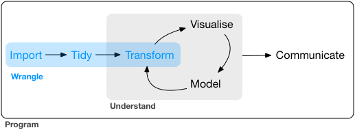
Tidying data

What is tidy data?

There are three interrelated rules which make a dataset tidy:

Each variable must have its own column.
Each observation must have its own row.
Each value must have its own cell.

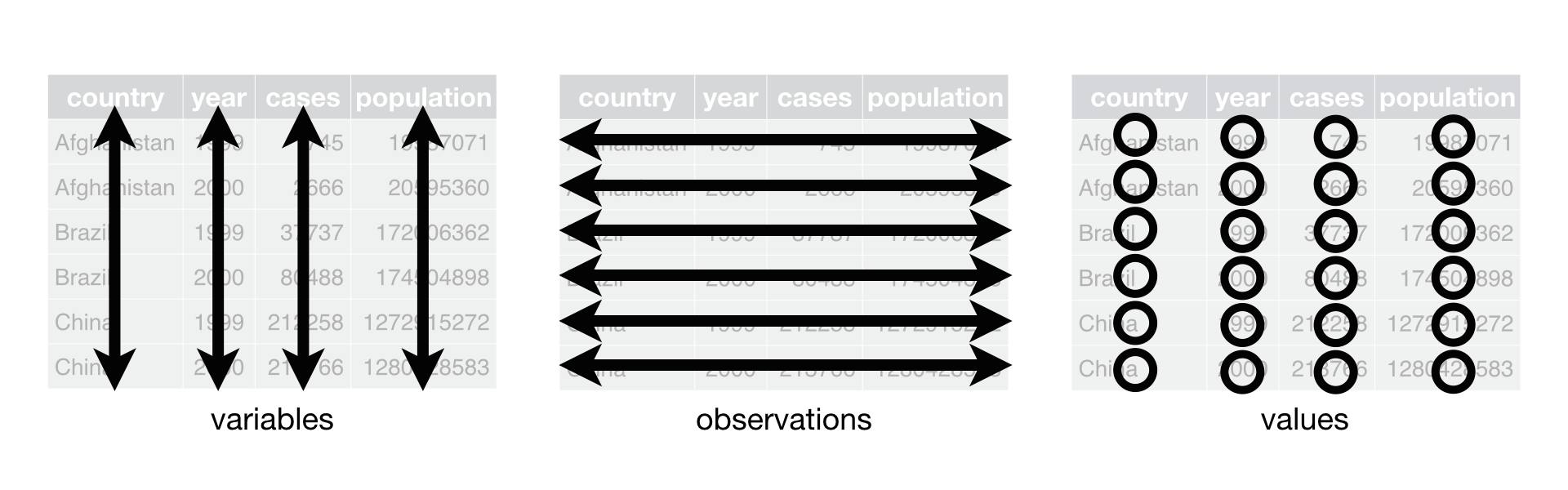Source: http://r4ds.had.co.nz

Datasets in different forms

Each dataset shows the same values of four variables country, year, population, and number of TB cases, but each dataset organises the values in a different way.

table1

## # A tibble: 6 x 4
##   country      year  cases population
##   <chr>       <int>  <int>      <int>
## 1 Afghanistan  1999    745   19987071
## 2 Afghanistan  2000   2666   20595360
## 3 Brazil       1999  37737  172006362
## 4 Brazil       2000  80488  174504898
## 5 China        1999 212258 1272915272
## 6 China        2000 213766 1280428583

table2

## # A tibble: 12 x 4
##    country      year type            count
##    <chr>       <int> <chr>           <int>
##  1 Afghanistan  1999 cases             745
##  2 Afghanistan  1999 population   19987071
##  3 Afghanistan  2000 cases            2666
##  4 Afghanistan  2000 population   20595360
##  5 Brazil       1999 cases           37737
##  6 Brazil       1999 population  172006362
##  7 Brazil       2000 cases           80488
##  8 Brazil       2000 population  174504898
##  9 China        1999 cases          212258
## 10 China        1999 population 1272915272
## 11 China        2000 cases          213766
## 12 China        2000 population 1280428583

In this example, only table1 is tidy. It’s the only representation where each column is a variable.

table3

## # A tibble: 6 x 3
##   country      year rate             
## * <chr>       <int> <chr>            
## 1 Afghanistan  1999 745/19987071     
## 2 Afghanistan  2000 2666/20595360    
## 3 Brazil       1999 37737/172006362  
## 4 Brazil       2000 80488/174504898  
## 5 China        1999 212258/1272915272
## 6 China        2000 213766/1280428583

table4a

## # A tibble: 3 x 3
##   country     `1999` `2000`
## * <chr>        <int>  <int>
## 1 Afghanistan    745   2666
## 2 Brazil       37737  80488
## 3 China       212258 213766

table4b

## # A tibble: 3 x 3
##   country         `1999`     `2000`
## * <chr>            <int>      <int>
## 1 Afghanistan   19987071   20595360
## 2 Brazil       172006362  174504898
## 3 China       1272915272 1280428583

Why tidy data?

If you pick one consistent way of storing data, then you can reuse the same tools.
R is naturally vectorized. Most built-in R functions work with vectors of values.
dplyr, ggplot2, and other packages in the tidyverse are designed to work with tidy data.

Why you need to know how to tidy data?

You cannot assume data will come in as tidy. In fact, most data is not.
Many people aren’t familiar with the principles of tidy data.
Data is often organised to facilitate some use other than analysis, e.g. storage efficiency, compactness or ease of data entry.

This means for most real analyses, you’ll need to do some tidying.

The `tidyr` package

Tidy datasets are all alike, but every messy dataset is messy in its own way.
–– Hadley Wickham

In the tidyverse, tidying data is done with tidyr package.

The same data can be represented in many different ways. Some are more practical than others.

Spreading, gathering, separating and uniting columns

First step. Determine what are the variables and what are the observations.

Second step. Often, you need to deal with some of the following issues:

One variable is spread across multiple columns $\implies$ need to gather().
One observation might be scattered across multiple rows $\implies$ need to spread().
One column contains values fore multiple variables $\implies$ need to separate().
Multiple columns store information on a single variable $\implies$ need to unite().

tidyr can help you solve these problems.

Gathering

Common problem: some column names are not the names, but the values of a variable.

table4a

## # A tibble: 3 x 3
##   country     `1999` `2000`
## * <chr>        <int>  <int>
## 1 Afghanistan    745   2666
## 2 Brazil       37737  80488
## 3 China       212258 213766

gather() makes wide tables narrower and longer:

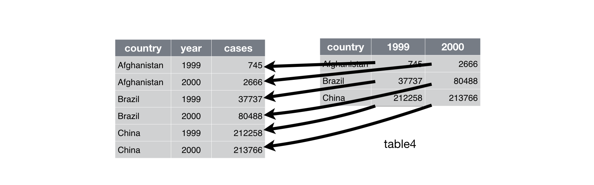
Gathering

To tidy up table4a, we need to gather() those columns into a new pair of variables. We need three pieces of information to do this:

The set of columns that represent values, not variables.
The name for the variable whose values are given in these columns’ names (the key).
The name for the variable whose values are spread over these columns’ cells (the value).

table4a

## # A tibble: 3 x 3
##   country     `1999` `2000`
## * <chr>        <int>  <int>
## 1 Afghanistan    745   2666
## 2 Brazil       37737  80488
## 3 China       212258 213766

gather(table4a, `1999`:`2000`, key = year, value = cases)

## # A tibble: 6 x 3
##   country     year   cases
##   <chr>       <chr>  <int>
## 1 Afghanistan 1999     745
## 2 Brazil      1999   37737
## 3 China       1999  212258
## 4 Afghanistan 2000    2666
## 5 Brazil      2000   80488
## 6 China       2000  213766

Spreading

Spreading is the opposite of gathering, and you use it when an observation is scattered across multiple rows.

spread() makes long tables shorter and wider:

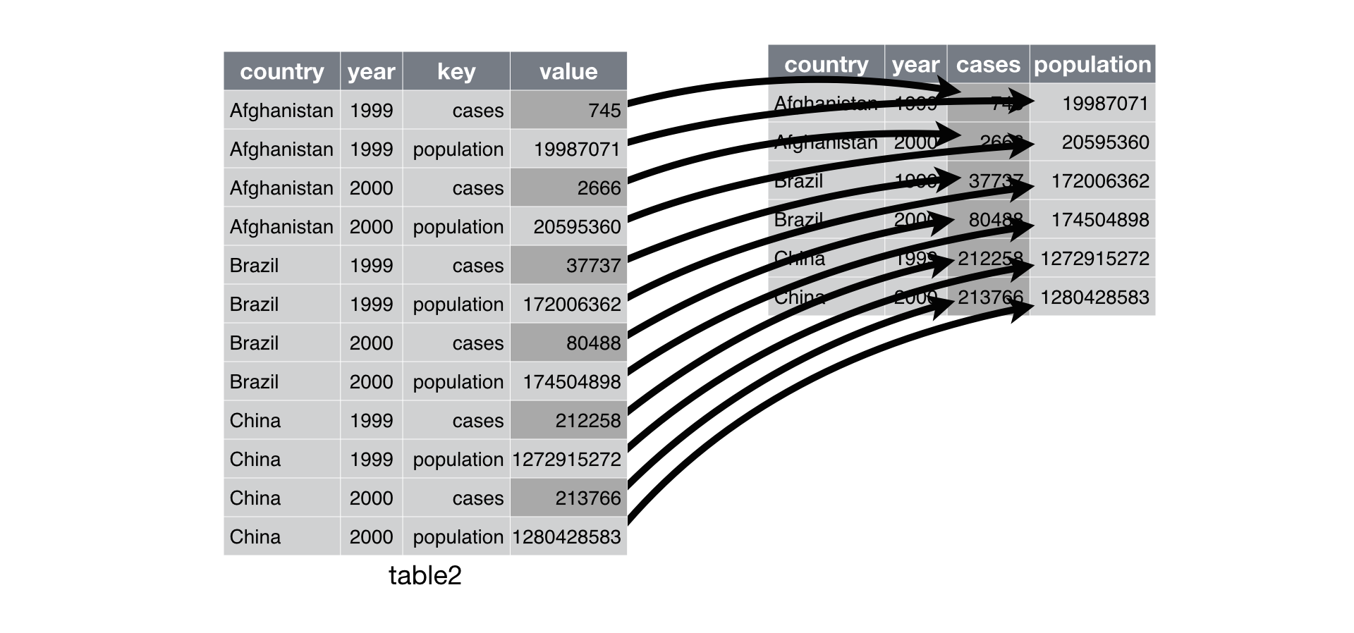
Spreading

To spread up table2, we only need two parameters:

The column that contains variable names (the key).
The column that contains values from multiple variables (the value).

table2

## # A tibble: 12 x 4
##    country      year type            count
##    <chr>       <int> <chr>           <int>
##  1 Afghanistan  1999 cases             745
##  2 Afghanistan  1999 population   19987071
##  3 Afghanistan  2000 cases            2666
##  4 Afghanistan  2000 population   20595360
##  5 Brazil       1999 cases           37737
##  6 Brazil       1999 population  172006362
##  7 Brazil       2000 cases           80488
##  8 Brazil       2000 population  174504898
##  9 China        1999 cases          212258
## 10 China        1999 population 1272915272
## 11 China        2000 cases          213766
## 12 China        2000 population 1280428583

spread(table2, key = type, value = count)

## # A tibble: 6 x 4
##   country      year  cases population
##   <chr>       <int>  <int>      <int>
## 1 Afghanistan  1999    745   19987071
## 2 Afghanistan  2000   2666   20595360
## 3 Brazil       1999  37737  172006362
## 4 Brazil       2000  80488  174504898
## 5 China        1999 212258 1272915272
## 6 China        2000 213766 1280428583

Separate

Sometimes, a dataset has a column with values corresponding to multiple variables.

We might want to split such a column into multiple new ones.

separate() makes narrow tables wider.

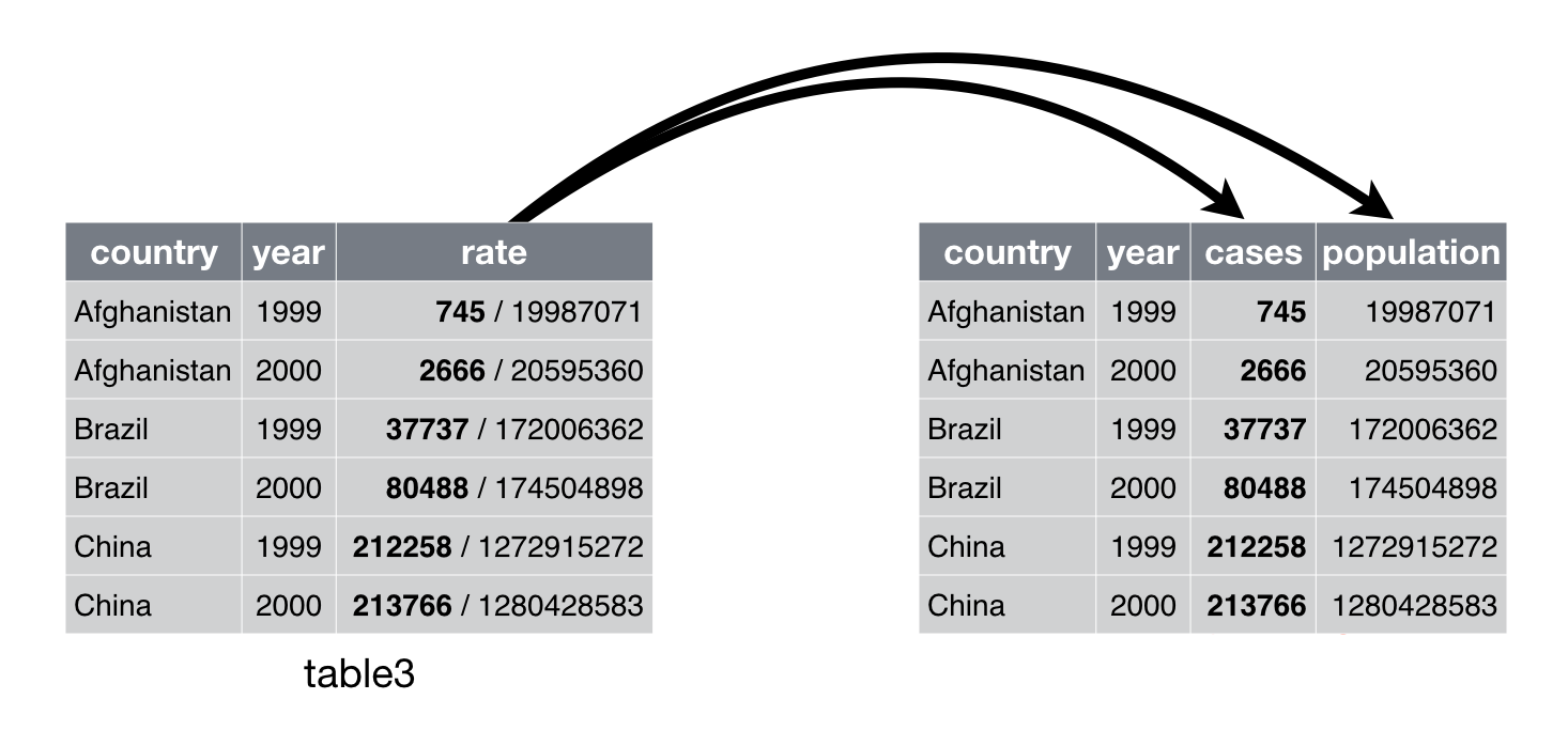
Separate

separate() splits one column into multiple columns wherever a separator appears.

table3

## # A tibble: 6 x 3
##   country      year rate             
## * <chr>       <int> <chr>            
## 1 Afghanistan  1999 745/19987071     
## 2 Afghanistan  2000 2666/20595360    
## 3 Brazil       1999 37737/172006362  
## 4 Brazil       2000 80488/174504898  
## 5 China        1999 212258/1272915272
## 6 China        2000 213766/1280428583

separate(table3, col = rate, 
         into = c("cases", "population"))

## # A tibble: 6 x 4
##   country      year cases  population
##   <chr>       <int> <chr>  <chr>     
## 1 Afghanistan  1999 745    19987071  
## 2 Afghanistan  2000 2666   20595360  
## 3 Brazil       1999 37737  172006362 
## 4 Brazil       2000 80488  174504898 
## 5 China        1999 212258 1272915272
## 6 China        2000 213766 1280428583

Some important features of separate()

by default, it splits values wherever it sees a non-alphanumeric character. You can specify the separator.

separate(table3, rate, into = c("cases", "population"), sep = "/")

by default, it leaves the type of the column as is. You can ask it to convert to better types.

separate(table3, col = rate, into = c("cases", "population"), convert = T)

Unite

unite() is the opposite of separate():
it combines multiple columns into a single column.

unite() makes wider tables narrower.

Unite

unite() takes arguments:

a tibble (or data.frame)
the name of the new column
names of columns to be combined
a separator used when uniting the columns

table5

## # A tibble: 6 x 4
##   country     century year  rate             
## * <chr>       <chr>   <chr> <chr>            
## 1 Afghanistan 19      99    745/19987071     
## 2 Afghanistan 20      00    2666/20595360    
## 3 Brazil      19      99    37737/172006362  
## 4 Brazil      20      00    80488/174504898  
## 5 China       19      99    212258/1272915272
## 6 China       20      00    213766/1280428583

unite(table5, col = full_year, century, year, 
      sep = "")

## # A tibble: 6 x 3
##   country     full_year rate             
##   <chr>       <chr>     <chr>            
## 1 Afghanistan 1999      745/19987071     
## 2 Afghanistan 2000      2666/20595360    
## 3 Brazil      1999      37737/172006362  
## 4 Brazil      2000      80488/174504898  
## 5 China       1999      212258/1272915272
## 6 China       2000      213766/1280428583

Transforming data

The `dplyr` package

The dplyr package is also a part of the core tidyverse, which:

Introduces a grammar of data manipulation.
Gives a code-efficient for way for data exploration and transformation.
Is fast on data frames (written in C++): has speed of C and ease of R.
Intuitive to write and easy to read, esp. when using the chaining syntax.

You should use dplyr even as a beginner R user, and here is why.

`dplyr` verbs (functions)

dplyr utilities handle the vast majority of your data manipulation needs:

filter() - for picking observations by their values,
select() - for picking variables by their names,
arrange() - for reorder the rows,
mutate() - for creating new variables with functions on existing variables,
summarise() - for collapse many values down to a single summary.

All of the above can be done using base R functions, but they would be less computationally efficient, and require writing more lines of (ugly) code.

The structure of `dplyr` functions

All verbs work similarly:

The first argument is a tibble (or data frame)
The subsequent ones describe what to do, using the variable names
The result is a new tibble

Learn more about dplyr from a turtorial written by its creator, Hadley Wickham.

The movie industry dataset

movies.csv contains information on last three decades of movies.

The data has been scraped from the IMDb website and can be accessed from a github repo.

url <- "https://raw.githubusercontent.com/Juanets/movie-stats/master/movies.csv"
movies <- read_csv(url)
movies

## # A tibble: 6,820 x 15
##    budget company country director genre  gross name  rating released runtime
##     <dbl> <chr>   <chr>   <chr>    <chr>  <dbl> <chr> <chr>  <chr>      <int>
##  1 8.00e6 Columb… USA     Rob Rei… Adve… 5.23e7 Stan… R      1986-08…      89
##  2 6.00e6 Paramo… USA     John Hu… Come… 7.01e7 Ferr… PG-13  1986-06…     103
##  3 1.50e7 Paramo… USA     Tony Sc… Acti… 1.80e8 Top … PG     1986-05…     110
##  4 1.85e7 Twenti… USA     James C… Acti… 8.52e7 Alie… R      1986-07…     137
##  5 9.00e6 Walt D… USA     Randal … Adve… 1.86e7 Flig… PG     1986-08…      90
##  6 6.00e6 Hemdale UK      Oliver … Drama 1.39e8 Plat… R      1987-02…     120
##  7 2.50e7 Henson… UK      Jim Hen… Adve… 1.27e7 Laby… PG     1986-06…     101
##  8 6.00e6 De Lau… USA     David L… Drama 8.55e6 Blue… R      1986-10…     120
##  9 9.00e6 Paramo… USA     Howard … Come… 4.05e7 Pret… PG-13  1986-02…      96
## 10 1.50e7 SLM Pr… USA     David C… Drama 4.05e7 The … R      1986-08…      96
## # … with 6,810 more rows, and 5 more variables: score <dbl>, star <chr>,
## #   votes <int>, writer <chr>, year <int>

`filter()`: retain rows matching a criteria

filter() allows you to subset observations based on their values.

# note: both comma and "&" represent AND condition
filter(movies, genre == "Comedy", director == "Woody Allen")

## # A tibble: 27 x 15
##    budget company country director genre  gross name  rating released runtime
##     <dbl> <chr>   <chr>   <chr>    <chr>  <dbl> <chr> <chr>  <chr>      <int>
##  1 6.40e6 Orion … USA     Woody A… Come… 4.01e7 Hann… PG-13  1986-03…     107
##  2 1.60e7 Orion … USA     Woody A… Come… 1.48e7 Radi… PG     1987-01…      88
##  3 1.90e7 Jack R… USA     Woody A… Come… 1.83e7 Crim… PG-13  1989-11…     104
##  4 1.50e7 Touchs… USA     Woody A… Come… 1.08e7 New … PG     1989-03…     124
##  5 1.20e7 Orion … USA     Woody A… Come… 7.33e6 Alice PG-13  1991-01…     106
##  6 1.40e7 Orion … USA     Woody A… Come… 2.74e6 Shad… PG-13  1992-03…      85
##  7 2.00e7 TriSta… USA     Woody A… Come… 1.06e7 Husb… R      1992-09…     103
##  8 1.35e7 TriSta… USA     Woody A… Come… 1.13e7 Manh… PG     1993-08…     104
##  9 2.00e7 Miramax USA     Woody A… Come… 1.34e7 Bull… R      1995-02…      98
## 10 1.50e7 Sweetl… USA     Woody A… Come… 6.70e6 Migh… R      1995-11…      95
## # … with 17 more rows, and 5 more variables: score <dbl>, star <chr>,
## #   votes <int>, writer <chr>, year <int>

# base R approach would be more wordy:
movies[movies$genre == "Comedy" & movies$director == "Woody Allen", ]

Package dplyr executes the filtering and returns a new data frame. It never modifies the original one.

Logical operators

Multiple arguments to filter() are combined with “and”: all expressions must be true, for a row to be included in the output. For other types of combinations, you’ll need to use Boolean operators yourself: & is “and”, | is “or”, and ! is “not”:

Source: R for data science

# Using AND operator
filter(movies, country == "USA", budget > 2.5e8) 
# same as filter(movies, country == "USA" & budget > 2.5e8)

# Using OR operator
filter(movies, country == "USA" | budget > 2.5e8)

# Using xor()
filter(movies, xor(score > 9, budget > 2.5e8))

# you can also use %in% operator
filter(movies, country %in% c("Peru", "Colombia", "Chile"))

## # A tibble: 8 x 15
##   budget company country director genre  gross name  rating released runtime
##    <dbl> <chr>   <chr>   <chr>    <chr>  <dbl> <chr> <chr>  <chr>      <int>
## 1 0.     Concor… Peru    "August… Acti… 4.11e5 Ultr… R      1990-03…     100
## 2 4.50e7 Warner… Peru    Luis Ll… Acti… 5.74e7 The … R      1994-10…     110
## 3 3.00e6 HBO Fi… Colomb… Joshua … Crime 6.52e6 Mari… R      2004-08…     101
## 4 0.     Partic… Chile   "Pablo … Drama 2.34e6 No    R      2012-11…     118
## 5 2.60e7 Alcon … Chile   Patrici… Biog… 1.22e7 Los … PG-13  2015-11…     127
## 6 1.40e6 Buffal… Colomb… Ciro Gu… Adve… 1.33e6 Embr… NOT R… 2015-05…     125
## 7 9.00e6 Fox Se… Chile   "Pablo … Biog… 1.40e7 Jack… R      2016-12…     100
## 8 0.     AZ Fil… Chile   "Pablo … Biog… 9.39e5 Neru… R      2017-03…     107
## # … with 5 more variables: score <dbl>, star <chr>, votes <int>, writer <chr>,
## #   year <int>

`select()`: pick columns by name

select() let’s you choose a subset variables, specified by name.

Note, there is no need for quotation marks in dplyr:

# dplyr approach
select(movies, name, country, year, genre)

## # A tibble: 6,820 x 4
##    name                     country  year genre    
##    <chr>                    <chr>   <int> <chr>    
##  1 Stand by Me              USA      1986 Adventure
##  2 Ferris Bueller's Day Off USA      1986 Comedy   
##  3 Top Gun                  USA      1986 Action   
##  4 Aliens                   USA      1986 Action   
##  5 Flight of the Navigator  USA      1986 Adventure
##  6 Platoon                  UK       1986 Drama    
##  7 Labyrinth                UK       1986 Adventure
##  8 Blue Velvet              USA      1986 Drama    
##  9 Pretty in Pink           USA      1986 Comedy   
## 10 The Fly                  USA      1986 Drama    
## # … with 6,810 more rows

# base R approach would be:
movies[, c("name", "year", "genre")]

select(movies, name, genre:score) # use colon to select contiguous columns,

## # A tibble: 6,820 x 7
##    name                     genre         gross rating released   runtime score
##    <chr>                    <chr>         <dbl> <chr>  <chr>        <int> <dbl>
##  1 Stand by Me              Adventure  52287414 R      1986-08-22      89   8.1
##  2 Ferris Bueller's Day Off Comedy     70136369 PG-13  1986-06-11     103   7.8
##  3 Top Gun                  Action    179800601 PG     1986-05-16     110   6.9
##  4 Aliens                   Action     85160248 R      1986-07-18     137   8.4
##  5 Flight of the Navigator  Adventure  18564613 PG     1986-08-01      90   6.9
##  6 Platoon                  Drama     138530565 R      1987-02-06     120   8.1
##  7 Labyrinth                Adventure  12729917 PG     1986-06-27     101   7.4
##  8 Blue Velvet              Drama       8551228 R      1986-10-23     120   7.8
##  9 Pretty in Pink           Comedy     40471663 PG-13  1986-02-28      96   6.8
## 10 The Fly                  Drama      40456565 R      1986-08-15      96   7.5
## # … with 6,810 more rows

select(movies, -(star:writer))    # To drop columns use a minus, "-"

## # A tibble: 6,820 x 12
##    budget company country director genre  gross name  rating released runtime
##     <dbl> <chr>   <chr>   <chr>    <chr>  <dbl> <chr> <chr>  <chr>      <int>
##  1 8.00e6 Columb… USA     Rob Rei… Adve… 5.23e7 Stan… R      1986-08…      89
##  2 6.00e6 Paramo… USA     John Hu… Come… 7.01e7 Ferr… PG-13  1986-06…     103
##  3 1.50e7 Paramo… USA     Tony Sc… Acti… 1.80e8 Top … PG     1986-05…     110
##  4 1.85e7 Twenti… USA     James C… Acti… 8.52e7 Alie… R      1986-07…     137
##  5 9.00e6 Walt D… USA     Randal … Adve… 1.86e7 Flig… PG     1986-08…      90
##  6 6.00e6 Hemdale UK      Oliver … Drama 1.39e8 Plat… R      1987-02…     120
##  7 2.50e7 Henson… UK      Jim Hen… Adve… 1.27e7 Laby… PG     1986-06…     101
##  8 6.00e6 De Lau… USA     David L… Drama 8.55e6 Blue… R      1986-10…     120
##  9 9.00e6 Paramo… USA     Howard … Come… 4.05e7 Pret… PG-13  1986-02…      96
## 10 1.50e7 SLM Pr… USA     David C… Drama 4.05e7 The … R      1986-08…      96
## # … with 6,810 more rows, and 2 more variables: score <dbl>, year <int>

`select()` helpers

You can use the following functions to help select the columns:

starts_with()
ends_with()
contains()
matches() (matches a regular expression)
num_range("x", 1:4): pickes variables x1, x2, x3, x4

Examples:

select(movies, starts_with("r"))
select(movies, ends_with("e"))
select(movies, contains("re"))

`arrange()`: reorder rows

arrange() takes a data frame and a set of column names to order by.
For descending order, use the function desc() around the column name.

print(arrange(movies, runtime), n = 4)

## # A tibble: 6,820 x 15
##   budget company country director genre  gross name  rating released runtime
##    <dbl> <chr>   <chr>   <chr>    <chr>  <dbl> <chr> <chr>  <chr>      <int>
## 1 0.     Iwerks… France  Jean-Ja… Adve… 1.51e7 Wing… G      1996-09…      50
## 2 1.25e7 Univer… USA     Don Blu… Anim… 4.81e7 The … G      1988-11…      69
## 3 6.00e3 Next W… UK      Christo… Crime 4.85e4 Foll… R      1999-11…      69
## 4 0.     Hyperi… USA     Bruce W… Anim… 8.44e6 "B\x… PG-13  1992-07…      70
## # … with 6,816 more rows, and 5 more variables: score <dbl>, star <chr>,
## #   votes <int>, writer <chr>, year <int>

# use `desc` for descending
print(arrange(movies, desc(budget)), n = 4)

## # A tibble: 6,820 x 15
##   budget company country director genre  gross name  rating released runtime
##    <dbl> <chr>   <chr>   <chr>    <chr>  <dbl> <chr> <chr>  <chr>      <int>
## 1 3.00e8 Walt D… USA     Gore Ve… Acti… 3.09e8 Pira… PG-13  2007-05…     169
## 2 2.60e8 Walt D… USA     Nathan … Anim… 2.01e8 Tang… PG     2010-11…     100
## 3 2.58e8 Columb… USA     Sam Rai… Acti… 3.37e8 Spid… PG-13  2007-05…     139
## 4 2.50e8 Warner… UK      David Y… Adve… 3.02e8 Harr… PG     2009-07…     153
## # … with 6,816 more rows, and 5 more variables: score <dbl>, star <chr>,
## #   votes <int>, writer <chr>, year <int>

`mutate()`: add new variables

mutate() adds new columns that are a function of the existing ones

movies <- mutate(movies, profit = gross - budget)
select(movies, name, gross, budget, profit)

## # A tibble: 6,820 x 4
##    name                         gross   budget     profit
##    <chr>                        <dbl>    <dbl>      <dbl>
##  1 Stand by Me               52287414  8000000   44287414
##  2 Ferris Bueller's Day Off  70136369  6000000   64136369
##  3 Top Gun                  179800601 15000000  164800601
##  4 Aliens                    85160248 18500000   66660248
##  5 Flight of the Navigator   18564613  9000000    9564613
##  6 Platoon                  138530565  6000000  132530565
##  7 Labyrinth                 12729917 25000000  -12270083
##  8 Blue Velvet                8551228  6000000    2551228
##  9 Pretty in Pink            40471663  9000000   31471663
## 10 The Fly                   40456565 15000000   25456565
## # … with 6,810 more rows

To discard old variables, use transmute() instead of mutate().

# base R approach to create a new variable 'profit'
movies$profit <- movies$gross - movies$budget

# Generating multiple new variables
movies <- mutate(
  movies, 
  profit = gross - budget, 
  gross_in_mil = gross/10^6,
  budget_in_mil = budget/10^6,
  profit_in_mil = profit/10^6
)
select(movies, name, year, country, contains("_in_mil"), profit)

## # A tibble: 6,820 x 7
##    name          year country gross_in_mil budget_in_mil profit_in_mil   profit
##    <chr>        <int> <chr>          <dbl>         <dbl>         <dbl>    <dbl>
##  1 Stand by Me   1986 USA            52.3            8           44.3    4.43e7
##  2 Ferris Buel…  1986 USA            70.1            6           64.1    6.41e7
##  3 Top Gun       1986 USA           180.            15          165.     1.65e8
##  4 Aliens        1986 USA            85.2           18.5         66.7    6.67e7
##  5 Flight of t…  1986 USA            18.6            9            9.56   9.56e6
##  6 Platoon       1986 UK            139.             6          133.     1.33e8
##  7 Labyrinth     1986 UK             12.7           25          -12.3   -1.23e7
##  8 Blue Velvet   1986 USA             8.55           6            2.55   2.55e6
##  9 Pretty in P…  1986 USA            40.5            9           31.5    3.15e7
## 10 The Fly       1986 USA            40.5           15           25.5    2.55e7
## # … with 6,810 more rows

Any vectorized function can be used with mutate(), including:

arithmetic operators (+,-,*,/, %, %%),
logical operators (<,<=,>,>=,==,!=),
logarithmic and exponential transfomations (log, log10, exp),
offsets (lead, lag),
cummulative rolling aggregates (cumsum, cumprod, cummin, cummax),
ranking (min_rank, percent_rank).

`summarise()`: reduce variables to values

summarize() can be used to aggregate data or to compute a summarizing value of interest.

summarise(movies, 
  tot_gross_in_bil = sum(gross)/1e9, 
  mean_gross_in_mil = mean(gross)/1e6, 
  mean_profit_in_mil = mean(profit)/1e6
)

## # A tibble: 1 x 3
##   tot_gross_in_bil mean_gross_in_mil mean_profit_in_mil
##              <dbl>             <dbl>              <dbl>
## 1             228.              33.5               8.92

summarize() is more useful on data previously grouped by one or more variables using group_by().

by_genre <- group_by(movies, genre)
summarize(by_genre, tot_gross_in_bil = sum(gross)/1e9, 
          mean_gross_in_mil = mean(gross)/1e6, 
          mean_profit_in_mil = mean(profit)/1e6)

Grouping and summarizing

Grouing allows you to compute summaries for each categories separately:

by_genre <- group_by(movies, genre)
summarize(
  by_genre, 
  tot_gross_in_bil = sum(gross)/1e9, 
  mean_gross_in_mil = mean(gross)/1e6, 
  mean_profit_in_mil = mean(profit)/1e6
)

## # A tibble: 17 x 4
##    genre     tot_gross_in_bil mean_gross_in_mil mean_profit_in_mil
##    <chr>                <dbl>             <dbl>              <dbl>
##  1 Action            74.8                56.2                7.30 
##  2 Adventure         20.9                53.3               16.0  
##  3 Animation         25.3                91.5               27.2  
##  4 Biography          8.62               24.0                7.05 
##  5 Comedy            53.5                25.7               10.8  
##  6 Crime             10.2                19.6                3.30 
##  7 Drama             25.2                17.5                4.19 
##  8 Family             0.118               8.44              -0.101
##  9 Fantasy            0.645              20.1                4.38 
## 10 Horror             7.12               25.7               13.8  
## 11 Musical            0.00809             2.02              -0.476
## 12 Mystery            1.38               36.3                9.47 
## 13 Romance            0.146               9.72               4.24 
## 14 Sci-Fi             0.308              23.7                6.79 
## 15 Thriller           0.0996              5.53              -0.356
## 16 War                0.00151             0.755              0.755
## 17 Western            0.0185              9.26               3.26

Elementary but useful summary functions

min(x), median(x), max(x), quantile(x, p)
n(), n_distinct(), sum(x), mean(x)
sum(x > 10), mean(x > 0)
sd(x), var(x)

Counting observations

tally() function can be used to generate a group frequency table, (number of observations in each category)

tally(group_by(movies, genre))

## # A tibble: 17 x 2
##    genre         n
##    <chr>     <int>
##  1 Action     1331
##  2 Adventure   392
##  3 Animation   277
##  4 Biography   359
##  5 Comedy     2080
##  6 Crime       522
##  7 Drama      1444
##  8 Family       14
##  9 Fantasy      32
## 10 Horror      277
## 11 Musical       4
## 12 Mystery      38
## 13 Romance      15
## 14 Sci-Fi       13
## 15 Thriller     18
## 16 War           2
## 17 Western       2

tally(group_by(movies, genre, country))

## # A tibble: 238 x 3
## # Groups:   genre [17]
##    genre  country            n
##    <chr>  <chr>          <int>
##  1 Action Aruba              1
##  2 Action Australia         12
##  3 Action Austria            1
##  4 Action Belgium            1
##  5 Action Brazil             2
##  6 Action Canada            26
##  7 Action China             13
##  8 Action Czech Republic     1
##  9 Action Denmark            2
## 10 Action France            41
## # … with 228 more rows

Window Functions

Aggregation functions such as mean(), n() return 1 value per group.
Window functions return multiple values per group, e.g. top_n(), lead and lag or cummean:

# rewrite more simply with the `top_n` function
movies2 <- select(movies, name, genre, country, year, budget, gross, profit, rating, score)
top2 <- top_n(group_by(movies2, genre), n = 2, wt = score)
arrange(top2, genre, year, score)

## # A tibble: 35 x 9
## # Groups:   genre [17]
##    name              genre   country    year budget  gross  profit rating score
##    <chr>             <chr>   <chr>     <int>  <dbl>  <dbl>   <dbl> <chr>  <dbl>
##  1 The Dark Knight   Action  USA        2008 1.85e8 5.35e8  3.50e8 PG-13    9  
##  2 Inception         Action  USA        2010 1.60e8 2.93e8  1.33e8 PG-13    8.8
##  3 The Lord of the … Advent… New Zeal…  2001 9.30e7 3.16e8  2.23e8 PG-13    8.8
##  4 The Lord of the … Advent… USA        2003 9.40e7 3.78e8  2.84e8 PG-13    8.9
##  5 The Lion King     Animat… USA        1994 4.50e7 3.13e8  2.68e8 G        8.5
##  6 Spirited Away     Animat… Japan      2001 1.90e7 1.01e7 -8.94e6 PG       8.6
##  7 Your name         Animat… Japan      2016 0.     5.02e6  5.02e6 PG       8.5
##  8 Schindler's List  Biogra… USA        1993 2.20e7 9.61e7  7.41e7 R        8.9
##  9 The Intouchables  Biogra… France     2011 0.     1.32e7  1.32e7 R        8.6
## 10 Forrest Gump      Comedy  USA        1994 5.50e7 3.30e8  2.75e8 PG-13    8.8
## # … with 25 more rows

Other useful functions in `dplyr`

# Renaming variables
print(rename(movies2, gross_revenue = gross), n = 5)

## # A tibble: 6,820 x 9
##   name          genre   country  year budget gross_revenue  profit rating score
##   <chr>         <chr>   <chr>   <int>  <dbl>         <dbl>   <dbl> <chr>  <dbl>
## 1 Stand by Me   Advent… USA      1986 8.00e6      52287414  4.43e7 R        8.1
## 2 Ferris Buell… Comedy  USA      1986 6.00e6      70136369  6.41e7 PG-13    7.8
## 3 Top Gun       Action  USA      1986 1.50e7     179800601  1.65e8 PG       6.9
## 4 Aliens        Action  USA      1986 1.85e7      85160248  6.67e7 R        8.4
## 5 Flight of th… Advent… USA      1986 9.00e6      18564613  9.56e6 PG       6.9
## # … with 6,815 more rows

# Unique values
distinct(movies2, rating)

## # A tibble: 13 x 1
##    rating       
##    <chr>        
##  1 R            
##  2 PG-13        
##  3 PG           
##  4 UNRATED      
##  5 Not specified
##  6 G            
##  7 NC-17        
##  8 NOT RATED    
##  9 TV-PG        
## 10 TV-MA        
## 11 B            
## 12 B15          
## 13 TV-14

# Using multiple variables, returns distinct variable combinations.
distinct(movies2, rating, genre)

## # A tibble: 83 x 2
##    rating  genre    
##    <chr>   <chr>    
##  1 R       Adventure
##  2 PG-13   Comedy   
##  3 PG      Action   
##  4 R       Action   
##  5 PG      Adventure
##  6 R       Drama    
##  7 PG-13   Adventure
##  8 PG-13   Action   
##  9 R       Crime    
## 10 UNRATED Comedy   
## # … with 73 more rows

Sampling observations

sample_n(movies, 5)                    # fixed number of rows, without replacement

## # A tibble: 5 x 19
##   budget company country director genre  gross name  rating released runtime
##    <dbl> <chr>   <chr>   <chr>    <chr>  <dbl> <chr> <chr>  <chr>      <int>
## 1 8.03e6 Davis … USA     Deran S… Acti… 3.41e6 Gunm… R      1994-02…      94
## 2 5.00e7 Young … UK      Peter W… Crime 2.77e7 Hann… R      2007-02…     121
## 3 1.60e8 Warner… USA     Gareth … Acti… 2.01e8 Godz… PG-13  2014-05…     123
## 4 3.50e7 Punch … USA     Robert … Come… 2.06e7 Boys… PG-13  2000-06…      94
## 5 0.     Mockin… USA     Robin S… Come… 3.57e6 The … PG-13  2007-10…     106
## # … with 9 more variables: score <dbl>, star <chr>, votes <int>, writer <chr>,
## #   year <int>, profit <dbl>, gross_in_mil <dbl>, budget_in_mil <dbl>,
## #   profit_in_mil <dbl>

sample_frac(movies, 0.005, replace=TRUE) # fraction of rows, with replacement

## # A tibble: 34 x 19
##    budget company country director genre  gross name  rating released runtime
##     <dbl> <chr>   <chr>   <chr>    <chr>  <dbl> <chr> <chr>  <chr>      <int>
##  1 0.     New Ar… USA     Courten… Come… 8.13e3 Just… R      2015-04…      95
##  2 7.00e6 Paramo… USA     Louis C… Come… 3.29e6 Poot… PG-13  2001-06…      81
##  3 5.00e6 Renais… Ireland Trevor … Come… 5.52e5 Twel… PG     1996-10…     134
##  4 1.50e7 Columb… USA     Richard… Drama 1.73e6 Litt… PG     1988-03…      98
##  5 0.     "Path\… France  Julian … Biog… 5.99e6 The … PG-13  2008-02…     112
##  6 0.     BBC Fi… UK      John Ma… Biog… 3.43e5 Love… UNRAT… 1998-10…      87
##  7 0.     Golden… Hong K… Michael… Adve… 3.96e5 Sex … R      1991-11…     100
##  8 1.50e7 New Li… USA     Sean Mc… Fami… 1.04e7 Rais… PG     2004-10…     100
##  9 5.50e7 Univer… USA     Jesse D… Come… 1.05e8 Amer… R      2003-08…      96
## 10 3.50e6 Incent… USA     Derek C… Drama 9.74e6 Blue… R      2011-01…     112
## # … with 24 more rows, and 9 more variables: score <dbl>, star <chr>,
## #   votes <int>, writer <chr>, year <int>, profit <dbl>, gross_in_mil <dbl>,
## #   budget_in_mil <dbl>, profit_in_mil <dbl>

Chaining operations

The `magrittr` package

The magrittr (to be pronounced with a sophisticated french accent) package has two aims: decrease development time and improve readability and maintainability of code

magrittr provides a “pipe”-like operator, %>%:

The %>% is used pipe values forward into an expression or function call.
In the pipe notation, you use x %>% f(y), rather than f(x, y).
This is similar to the Unix pipes, |, used to send the output of one program to another program for further processing.

columns <- 1:50
rnorm(500) %>%
  matrix(ncol = 50) %>%
  colSums() %>%
  plot(x = columns)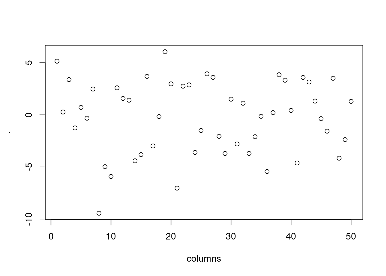

Chaining operations

Pipe operators used together with dplyr functions make a large difference as they semantically change your code in a way that makes it more intuitive to both read and write.
The pipes allow users to chain operators which reflects the sequential nature of data-processing tasks.
Chaining increases readability significantly when there are many commands
%>% operator is automatically imported into dplyr

Find movies from USA produced after 2010. (2) Group by genre and
compute the group mean gross revenue in million dollars. Then print the genre mean ‘gross’ revenue (4) arranged in a descending order:

# nesting 
arrange(
  summarise(
    group_by(
      filter(movies, 
             year > 2010, country == "USA"
      ),
      genre
    ),
    mean_gross = mean(gross)/10^6
  ),
  mean_gross
)

## # A tibble: 13 x 2
##    genre     mean_gross
##    <chr>          <dbl>
##  1 Thriller      0.0165
##  2 Drama        23.3   
##  3 Horror       27.7   
##  4 Sci-Fi       29.2   
##  5 Fantasy      30.7   
##  6 Crime        32.1   
##  7 Comedy       35.2   
##  8 Biography    40.6   
##  9 Mystery      49.5   
## 10 Romance      62.5   
## 11 Adventure    81.2   
## 12 Action       97.3   
## 13 Animation   152.

# chaining 
movies %>%
  filter(year > 2010, country == "USA") %>%
  group_by(genre) %>%
  summarise(mean_gross = mean(gross)/10^6) %>%
  arrange(mean_gross)

## # A tibble: 13 x 2
##    genre     mean_gross
##    <chr>          <dbl>
##  1 Thriller      0.0165
##  2 Drama        23.3   
##  3 Horror       27.7   
##  4 Sci-Fi       29.2   
##  5 Fantasy      30.7   
##  6 Crime        32.1   
##  7 Comedy       35.2   
##  8 Biography    40.6   
##  9 Mystery      49.5   
## 10 Romance      62.5   
## 11 Adventure    81.2   
## 12 Action       97.3   
## 13 Animation   152.

Exercises 2

Go to the “Lec3_Exercises.Rmd” file, which can be downloaded from the class website under the Lecture tab.
Complete Exercise 2.

Lecture 3: Importing and transforming data

CME/STATS 195

Lan Huong Nguyen

October 4, 2018

Contents

Importing data

Working Directory

Paths and directory names

Importing text data

The readr package

Comparison with base R

Reading comma-separated files

The read_csv() function

How readr parses data?

Potential difficulties

Locales

Parsing dates

Parsing times

Parsing numbers

Parsing real numbers

readr’s strategy for parsing files

When the default strategy fails

Examining what went wrong

Fixing the column specifications

Fixing the column specifications

Diagnosing problems

Importing other types of data

Exercise 1

Tidying data

What is tidy data?

Datasets in different forms

Why tidy data?

Why you need to know how to tidy data?

The tidyr package

Spreading, gathering, separating and uniting columns

Gathering

Gathering

Spreading

Spreading

Separate

Separate

Unite

Unite

Transforming data

The dplyr package

dplyr verbs (functions)

The structure of dplyr functions

The movie industry dataset

filter(): retain rows matching a criteria

Logical operators

select(): pick columns by name

select() helpers

arrange(): reorder rows

mutate(): add new variables

summarise(): reduce variables to values

Grouping and summarizing

Elementary but useful summary functions

Counting observations

Window Functions

Other useful functions in dplyr

Sampling observations

Chaining operations

The magrittr package

Chaining operations

Exercises 2

The `readr` package

The `read_csv()` function

How `readr` parses data?

`readr’s` strategy for parsing files

The `tidyr` package

The `dplyr` package

`dplyr` verbs (functions)

The structure of `dplyr` functions

`filter()`: retain rows matching a criteria

`select()`: pick columns by name

`select()` helpers

`arrange()`: reorder rows

`mutate()`: add new variables

`summarise()`: reduce variables to values

Other useful functions in `dplyr`

The `magrittr` package