Data Science Workflow

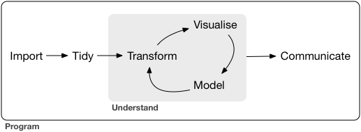
Data science is an exciting discipline that allows you to turn raw data into understanding, insight, and knowledge. ¹

tidyverse

# Install the package
install.packages("tidyverse")
# Load it into memory
library("tidyverse")

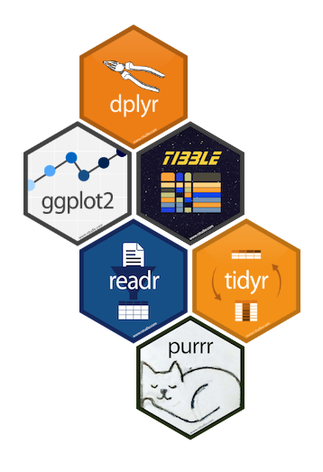
The tibble package

The tibble package is part of the core tidyverse.

Using tibbles

To use functions from tibble and other tidyverse packages:

# load it into memory
library(tidyverse)

Printing tibble is much nicer, and always fits into your window:

# e.g. a built-in dataset 'diamonds' is a tibble:
class(diamonds)

## [1] "tbl_df"     "tbl"        "data.frame"

diamonds

## # A tibble: 53,940 x 10
##    carat cut       color clarity depth table price     x     y     z
##    <dbl> <ord>     <ord> <ord>   <dbl> <dbl> <int> <dbl> <dbl> <dbl>
##  1 0.23  Ideal     E     SI2      61.5    55   326  3.95  3.98  2.43
##  2 0.21  Premium   E     SI1      59.8    61   326  3.89  3.84  2.31
##  3 0.23  Good      E     VS1      56.9    65   327  4.05  4.07  2.31
##  4 0.290 Premium   I     VS2      62.4    58   334  4.2   4.23  2.63
##  5 0.31  Good      J     SI2      63.3    58   335  4.34  4.35  2.75
##  6 0.24  Very Good J     VVS2     62.8    57   336  3.94  3.96  2.48
##  7 0.24  Very Good I     VVS1     62.3    57   336  3.95  3.98  2.47
##  8 0.26  Very Good H     SI1      61.9    55   337  4.07  4.11  2.53
##  9 0.22  Fair      E     VS2      65.1    61   337  3.87  3.78  2.49
## 10 0.23  Very Good H     VS1      59.4    61   338  4     4.05  2.39
## # … with 53,930 more rows

Using tibbles

Creating tibbles is similar to data.frames, but no strict rules on column names:

(tb <- tibble(x = 1:5, y = 1,z = x ^ 2 + y, `:)` =  "smile"))

## # A tibble: 5 x 4
##       x     y     z `:)` 
##   <int> <dbl> <dbl> <chr>
## 1     1     1     2 smile
## 2     2     1     5 smile
## 3     3     1    10 smile
## 4     4     1    17 smile
## 5     5     1    26 smile

Subsetting tibbles is stricter than subsetting data.frames, and ALWAYS returns objects with expected class: a single [ returns a tibble, a double[[ returns a vector.

class(diamonds$carat)

## [1] "numeric"

class(diamonds[["carat"]])

## [1] "numeric"

class(diamonds[, "carat"])

## [1] "tbl_df"     "tbl"        "data.frame"

More on tibbles

You can read more about other tibble features by calling on your R console:

vignette("tibble")

R Markdown

R Markdown was designed to be used:

• for communicating your conclusions with people who do not want to focus on the code behind the analysis.

• for collaborating with other data scientists, interested in both conclusions, and the code.

• as a modern day lab notebook for data science, where you can capture both your work and your thought process.

R Markdown sourse files

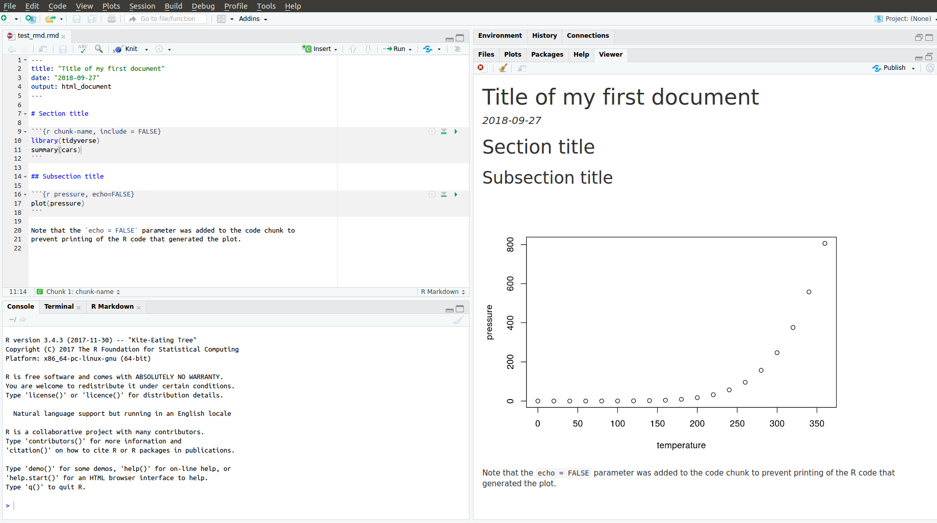
R Markdown files are a plain text files with “.Rmd” extension.

    ---
    title: "Title of my first document"
    date: "2018-09-27"
    output: html_document
    ---
    
    # Section title
    
    ```{r chunk-name, include = FALSE}
    library(tidyverse)
    summary(cars)
    ```
    
    ## Subsection title
    
    ```{r pressure, echo=FALSE}
    plot(pressure)
    ```
    
    Note that the `echo = FALSE` parameter was added to the code chunk to 
    prevent printing of the R code that generated the plot.

The documents must contain YAML header marked with dashes. You can ass both code chunks and plain text. Sections and subsections are marked with hashtags.

Compiling R Markdown files

To produce a complete report containing all text, code, and results:

• In RStudio, click on “Knit” or press Cmd/Ctrl + Shift + K.

• From the R command line, type rmarkdown::render(“filename.Rmd”)

This will display the report in the viewer pane, and create a self-contained HTML file that you can share with others.

After compiling the R Markdown document from the previous slide, you get this html.

Viewing the report in RStudio

YAML header

A YAML header is a set of key: value pairs at the start of your file. Begin and end the header with a line of three dashes (- - -), e.g.

---
title: "Untitled"
author: "Anonymous"
output: html_document
---

You can tell R Markdown what type of document you want to render: html_document (default), pdf_document, word_document, beamer_presentation etc.

You can print a table of contents (toc) with the following:

---
title: "Untitled"
author: "Anonymous"
output: 
  html_document:
    toc: true
---

Text in R Markdown

In “.Rmd” files, prose is written in Markdown, a lightweight markup language with plain text files formating syntax.

Section headers/titles:

# 1st Level Header

## 2nd Level Header

### 3rd Level Header

Text formatting:

*italic* or _italic_
**bold** __bold__

`code`
superscript^2^ and subscript~2~

Text in R Markdown

Lists:

* unordered list
* item 2
    + sub-item 1
    + sub-item 2 
    
1. ordered list 
1. item 2. The numbers are incremented automatically in the output.

Links and images:

<http://example.com> 

[linked phrase](http://example.com)

![optional caption text](path/to/img.png)

Text in R Markdown

Tables:

Table Header | Second Header
-------------| -------------
Cell 1       | Cell 2
Cell 3       | Cell 4 

Math formulae

$\alpha$ is the first letter of the Greek alphabet.

Using $$ prints a centered equation in the new line.

$$\sqrt{\alpha^2 + \beta^2} = \frac{\gamma}{2}$$

Code chunks

In R Markdown R code must go inside code chunks, e.g.:

  ```{r chunk-name}
      x <- runif(10)
      y <- 10 * x + 4
      plot(x, y)
  ```

Keyboard shortcuts:

• Insert a new code chunk: Ctrl/Cmd + Alt + I

• Run current chunk: Ctrl/Cmd + Shift + Enter

• Run current line (where the cursor is): Ctrl/Cmd + Enter

Chunk Options:

Chunk output can be customized with options supplied to chunk header. Some non-default options are:

• eval = FALSE : prevents code from being evaluated
• include = FALSE : runs the code, but hides code and its output in the final document
• echo = FALSE : hides the code, but not the results, in the final document
• message = FALSE : hides messages
• warning = FALSE : hides warnings
• results = ‘hide’ : hides printed output
• fig.show = ‘hide’ : hides plots
• error = TRUE : does not stop rendering if error occurs

Inline code

You can evealuate R code in a middle of your text:

  There are 26 in the alphabet, and 12 months in each year. 
  Today, there are `as.Date("2019-08-23") - Sys.Date()` days left till my next birthday.

There are 26 in the alphabet, and 12 months in a year. Today, there are 325 days left till my next birthday.

More on R Markdown

R Markdown is relatively young, and growing rapidly.

Official R Markdown website: (http://rmarkdown.rstudio.com)

Further reading and references:

• https://bookdown.org/yihui/rmarkdown/
• http://www.stat.cmu.edu/~cshalizi/rmarkdown
• https://www.rstudio.com/resources/cheatsheets/

Some R Markdown advice

• See your future self as a collaborator.
• Ensure each notebook has a descriptive title and name.
• Use the header date to record start time
• Keep track of failed attempts
• If you discover an error in a data file, write code to fix it.
• Regularly knit the notebook
• Use random seeds before sampling.
• Keep track the versions of the packages you use, e.g. by including sessionInfo() command at the end of your document.

All the above will help you increase the reproduciblity of your work.

Naming conventions

The first step of programming is naming things.
In the “Hadley Wickam” R style convention:

File names are meaningful. Script files end with “.R”, and R Markdown with “.Rmd”

# Good
fit-models.R
utility-functions.R

# Bad (works but does not follow style convention)
foo.r
stuff.r

# Good
day_one
day_1

# Bad (works but does not follow style convention)
first_day_of_the_month
DayOne

Spacing

Spacing around all infix operators (=, +, -, <-, etc.):

average <- mean(feet / 12 + inches, na.rm = TRUE)     # Good
average<-mean(feet/12+inches,na.rm=TRUE)              # Bad

Spacing before left parentheses, except in a function call

# Good
if (debug) do(x)
plot(x, y)

# Bad
if(debug)do(x)
plot (x, y)

# Good
x <- 1 + 2

# Bad (works but does not follow style convention)
x = 1 + 2

Curly braces

# Good
if (y < 0 && debug) {
  message("Y is negative")
}
if (y == 0) {
  log(x)
} else {
  y ^ x
}

# Bad
if (y < 0 && debug)
message("Y is negative")

if (y == 0) {
  log(x)
} 
else {
  y ^ x
}

if (y < 0 && debug) message("Y is negative")

Comments and documentation

Comment your code!

# 'get_answer' returns the answer to life, the universe and everything else.
get_answer <- function(){ return(42)}    # This is a comment

Comments are not subtitles, i.e. don’t repeat the code in the comments.

# Bad comments:
# Loop through all bananas in the bunch
for(banana in bunch) {
  # make the monkey eat one banana
  MonkeyEat(b)  
}

Use dashes to separate blocks of code:

# Generate Data ---------------------------
x <- rnorm(100)
y <- 12 * x + 5

# Plot Data -------------------------------
plot(x, y)

Booleans/logicals

# equal "==""
5 == 5

## [1] TRUE

# not equal: "!="" 
5 != 5 

## [1] FALSE

# greater than: ">""
5 > 4 

## [1] TRUE

# greater than or equal: ">="" (# similarly < and <=)
5 >= 5

## [1] TRUE

# You can combine multiple boolean expressions
TRUE & TRUE

## [1] TRUE

TRUE & FALSE 

## [1] FALSE

TRUE | FALSE

## [1] TRUE

!(TRUE)

## [1] FALSE

Booleans/logicals

In R if you combine 2 vectors of booleans, by each element then use &. Rember the recycling property for vectors.

c(TRUE, TRUE) & c(FALSE, TRUE)

## [1] FALSE  TRUE

c(5 < 4, 7 == 0, 1< 2) | c(5==5, 6> 2, !FALSE)

## [1] TRUE TRUE TRUE

c(TRUE, TRUE) & c(TRUE, FALSE, TRUE, FALSE)  # recycling

## [1]  TRUE FALSE  TRUE FALSE

Booleans/logicals

If we use double operators && or || is used only the first elements are compared:

c(TRUE, TRUE) && c(FALSE, TRUE)

## [1] FALSE

c(5 < 4, 7 == 0, 1< 2) || c(5==5, 6> 2, !FALSE)

## [1] TRUE

c(TRUE, TRUE) && c(TRUE, FALSE, TRUE, FALSE)

## [1] TRUE

Booleans/logicals

• Another possibility to combine booleans is to use all() or any() functions:

all(c(TRUE, FALSE, TRUE))

## [1] FALSE

any(c(TRUE, FALSE, TRUE))

## [1] TRUE

all(c(5 > -1, 3 >= 1, 1 < 1))

## [1] FALSE

any(c(5 > -1, 3 >= 1, 1 < 1))

## [1] TRUE

Control statements

• Control flow is the order in which individual statements, instructions or function calls of a program are evaluated.

• Control statements allow you to do more complicated tasks.

• Their execution results in a choice between which of two or more paths should be followed.
  • If / else
  • For
  • While

If statements

if (traffic_light == "green") {
  print("Go.")
}

if (traffic_light == "green") {
   print("Go.")
} else {
   print("Stay.")
}

if (traffic_light == "green") {
  print("Go.")
} else if (traffic_light == "yellow") {
  print("Get ready.")
} else {
  print("Stay.")
}

Switch statements

For very long sequence of if statements, use the switch() function

operator <- function(x, y, op) {
  switch(as.character(op),
    '+' = x + y,
    '-' = x - y,
    '*' = x * y,
    '/' = x / y,
  stop("Unknown op!")
  )
}

operator(2, 7, '+')

## [1] 9

operator(2, 7, '-')

## [1] -5

operator(2, 7, '/')

## [1] 0.2857143

operator(2, 7, "a")

## Error in operator(2, 7, "a"): Unknown op!

For loops

• A for loop is a statement which repeats the execution a block of code a given number of iterations.

for (i in 1:5){
  print(i^2)
}

## [1] 1
## [1] 4
## [1] 9
## [1] 16
## [1] 25

While loops

• Similar to for loops, but repeat the execution as long as the boolean condition supplied is TRUE.

i = 1
while(i <= 5) {
  cat("i =", i, "\n")
  i = i + 1
}

## i = 1 
## i = 2 
## i = 3 
## i = 4 
## i = 5

Next

for (i in 1:10) {
  if (i <= 5) {
    print("skip")
    next
  }
  cat(i, "is greater than 5.\n")
}

## [1] "skip"
## [1] "skip"
## [1] "skip"
## [1] "skip"
## [1] "skip"
## 6 is greater than 5.
## 7 is greater than 5.
## 8 is greater than 5.
## 9 is greater than 5.
## 10 is greater than 5.

for (i in 1:3) {
  cat("Outer-loop i: ", i, ".\n")
  for (j in 1:4) {
    if(j > i) {
      print("skip")
      next
    }
    cat("Inner-loop j:", j, ".\n")
  }
}

## Outer-loop i:  1 .
## Inner-loop j: 1 .
## [1] "skip"
## [1] "skip"
## [1] "skip"
## Outer-loop i:  2 .
## Inner-loop j: 1 .
## Inner-loop j: 2 .
## [1] "skip"
## [1] "skip"
## Outer-loop i:  3 .
## Inner-loop j: 1 .
## Inner-loop j: 2 .
## Inner-loop j: 3 .
## [1] "skip"

Break

• The break statement allows us to break out out of a for, while loop (of the smallest enclosing).
• The control is transferred to the first statement outside the inner-most loop.

for (i in 1:10)  {
  if (i == 6)  {
    print(paste("Coming out from for loop Where i = ", i))
    break
  }
  print(paste("i is now: ", i))
}

## [1] "i is now:  1"
## [1] "i is now:  2"
## [1] "i is now:  3"
## [1] "i is now:  4"
## [1] "i is now:  5"
## [1] "Coming out from for loop Where i =  6"

Exercise 1

• Go to “Lec2_Exercises.Rmd” in RStudio.

• Do Exercise 1.

What is a function in R?

• A function is a procedure/routine that performs a specific task.

• Functions are used to abstract components of larger program.

• Similarly to mathematical functions, they take some input and then do something to find the result.

• Functions allow you to automate common tasks in a more powerful and general way than copy-and-pasting.

• If you’ve copied and pasted a block of code more than twice, you should use a function instead.

Why should you use functions?

Functions become very useful as soon as your code becomes long enough.

• Functions will make your code easier to understand.
• Errors are less likely to occure and easier to fix.
• For repeated taskes, changes can be made once by editing a function and not many distant chunks of code. Example:

set.seed(1)
a <- rnorm(10); b <- rnorm(10); c <- rnorm(10); d <- rnorm(10)
# Bad
a <- (a - min(a, na.rm = TRUE)) /
  (max(a, na.rm = TRUE) - min(a, na.rm = TRUE))
b <- (b - min(b, na.rm = TRUE)) /
  (max(b, na.rm = TRUE) - min(b, na.rm = TRUE))
c <- (c - min(c, na.rm = TRUE)) /
  (max(b, na.rm = TRUE) - min(c, na.rm = TRUE))
d <- (d - min(d, na.rm = TRUE)) /
  (max(d, na.rm = TRUE) - min(d, na.rm = TRUE))

# Good
rescale_data <- function(x) {
  rng <- range(x, na.rm = TRUE)
  return((x - rng[1]) / (rng[2] - rng[1]))
}
a <- rescale_data(a)
b <- rescale_data(b)
c <- rescale_data(c)
d <- rescale_data(d)

Function Definition

• To define a function you assign a variable name to a function object.

• Functions take arguments, mandatory and optional.

• Provide the brief description of your function in comments before the function definition.

# Computes mean and standard deviation of a vector,
# and optionally prints the results.
summarize_data <- function(x, print=FALSE) {
  center <- mean(x)
  spread <- sd(x) 
  if (print) {
    cat("Mean =", center, "\n", 
        "SD   =", spread, "\n")
  }
  list(mean=center, sd=spread)
}

Calling functions

# without printing
x <- rnorm(n = 500, mean = 4, sd = 1) 
y <- summarize_data(x)

# with printing
y <- summarize_data(x, print = TRUE)

## Mean = 4.009679 
##  SD   = 1.01561

# Results are stored in list "y"
y$mean

## [1] 4.009679

y$sd

## [1] 1.01561

# The order of arguments does not matter if the names are specified
y <- summarize_data(print=FALSE, x = x)

Explicit return statements

The value returned by the function is usually the last statement it evaluates. You can choose to return early by using return(); this makes you code easier to read.

# Complicated function simplified by the use of early return statements
complicated_function <- function(x, y, z) {
  # Check some condition
  if (length(x) == 0 || length(y) == 0) {
    return(0)
  }
  # Complicated code here
}

Returning invisible objects can be done with invisible()

show_missings <- function(df) {
  cat("Missing values:", sum(is.na(df)), "\n")
  invisible(df)       # this result doesn’t get printed out
}

show_missings(mtcars)

## Missing values: 0

dim(show_missings(mtcars))

## Missing values: 0

## [1] 32 11

Environment

The environment of a function controls how R finds an object associated with a name.

f <- function(x) {
  x + y
}

R uses rules called lexical scoping to find the value associated with a name. Here, R will look for y in the environment where the function was defined

y <- 100
f(10)

## [1] 110

This behaviour attracts bugs. You should try to avoid using global variables.

apply, lapply, sapply functions

• The apply family functions, are functions which manipulate slices of data stored as matrices, arrays, lists and data-frames in a repetitive way.

• These functions avoid the explicit use of loops, and might be more computationally efficient, depending on how big a dataset is. For more details on runtimes see this link.

• apply allow you to perform operations with very few lines of code.

• The family comprises: apply, lapply , sapply, vapply, mapply, rapply, and tapply. The difference lies in the structure of input data and the desired format of the output).

apply function

apply operates on arrays/matrices.

In the example below we obtain column sums of matrix X.

(X <- matrix(sample(30), nrow = 5, ncol = 6))

##      [,1] [,2] [,3] [,4] [,5] [,6]
## [1,]   11   21   10   16    7   15
## [2,]   30   13   14   27   23    2
## [3,]   18    3    5    8    4   28
## [4,]    1   20    6   24   26   25
## [5,]   19    9   12   29   22   17

apply(X, MARGIN = 2 , FUN = sum)

## [1]  79  66  47 104  82  87

Note: that in a matrix MARGIN = 1 indicates rows and MARGIN = 2 indicates columns.

apply function

• apply can be used with user-defined functions:

# number entries < 15
apply(X, 2, function(x) 10*x + 2) 

##      [,1] [,2] [,3] [,4] [,5] [,6]
## [1,]  112  212  102  162   72  152
## [2,]  302  132  142  272  232   22
## [3,]  182   32   52   82   42  282
## [4,]   12  202   62  242  262  252
## [5,]  192   92  122  292  222  172

• a function can be defined outside apply(),

logColMeans <- function(x, eps = NULL) {
  if (!is.null(eps)) x <- x + eps
  return(mean(x))
}
apply(X, 2, logColMeans) 

## [1] 15.8 13.2  9.4 20.8 16.4 17.4

apply(X, 2, logColMeans, eps = 0.1) 

## [1] 15.9 13.3  9.5 20.9 16.5 17.5

lapply/sapply functions

• lapply() is used to repeatedly apply a function to elements of a sequential object such as a vector, list, or data-frame (applies to columns).

• The output is a list with the same number of elements as the input object.

# lapply returns a list
lapply(1:3, function(x) x^2)

## [[1]]
## [1] 1
## 
## [[2]]
## [1] 4
## 
## [[3]]
## [1] 9

• sapply is the same as lapply but returns a “simplified” output.

sapply(1:3, function(x) x^2)

## [1] 1 4 9

• like with apply(), user-defined functions can be used with sapply/lapply.

Functional Programming

The idea of passing a function to another function is extremely powerful idea, and it’s one of the behaviours that makes R a functional programming (FP) language.

The apply family of functions in base R are basically tools to extract out this duplicated code, so each common for loop pattern gets its own function.

The package purrr in tidyverse framework solves similar problems, more in line with the ‘tidyverse-philosophy’. We will learn in in following lectures.

Exercise 2 and 3

• Go back to “Lec2_Exercises.Rmd” in RStudio.

• Do Exercise 2 and 3.